KT 猫的介绍

Posted 2023-05-15

kt猫有动画片吗。谢谢

hello kitty
中英文名:凯蒂猫(KITTY WHITE)

匿称：Hello Kitty

性别：可爱小女孩 (漂亮的小女生)

生日：1974年11月1日

星座：天蝎座 (和原创作者相同)

血型：A型

出生地：英国伦敦

身高：5个苹果高

体重：3个苹果重

家庭成员：妈妈.爸爸.双包胎妹妹

性格：开朗活泼，温柔热心，调皮可爱，喜欢交朋友

专长：最擅长打网球， 钢琴也弹得非常好

最拿手厨艺：欧洲田园风手制小饼干

最喜欢的事物：喜欢听童话故事，收集各式各样美丽可爱的小装饰品，有糖果、小星星、小金鱼，尤其以蝴蝶结为最多，喜欢和许多好朋友一起到公园或森林去玩

最喜欢的食物：妈妈亲手做的苹果派&镇上面包屋叔叔的爱心面包

最喜欢的科目： 英语及音乐

最佳的代步工具：喜欢骑著粉红色的三轮脚踏车去公园玩耍

最有魅力的重点：全身上下充满可爱气息的KITTY， 最有吸引力的地方是左耳上戴著红色蝴蝶结， 还有一个圆圆的小尾巴

喜欢的颜色：红色，是跟她的蝴蝶结一样的颜色。

喜欢的服装：为了方便到处活动，活泼的KITTY，总喜欢穿着男性化的工人裤。但有时有会穿着美美的连身裙和洋装，非常地女性化喔!

最甜蜜的梦想：跟丹尼尔在一个浪漫的海边小教堂结婚

未来的愿望：希望长大后当一个伟大的诗人和钢琴家

Hello Kitty的家人

住在英国伦敦近郊小镇的红屋顶小白屋，是两层高的平房，离伦敦市中心 (泰晤士河) 20公里的地方。小镇上约有2万多人口，祖父母居住在附近一个森林里，只要一天的时间就足够步行过去。放假时，爸爸会开车戴著家人一起 去探望爷爷奶奶。Kitty的学校位于伦敦市，离家要4公里。Kitty每天都乘著巴士上学，只需过三个站即可到达。
爸爸PaPa

George White(佐治维特) 是一个可靠且又有幽默感的好爸爸，他十分重视家庭，非常疼爱小孩子，最爱抽大烟斗。

妈妈MaMa

Mary White(玛丽维特) 一个慈祥的妈妈，充满爱心和温柔，她是全能的家庭主妇，喜爱种花，烹饪和布置房间，Kitty最喜欢吃妈妈亲手做的苹果派。

咪咪(Mimmy)

Kitty的双胞胎妹妹，她头戴著粉黄色蝴蝶结，很讨人喜欢，个性很害羞也很恋家，喜爱跟奶奶学习作手工艺，常常会幻想长大成为一位幸福的新娘子。

爷爷(Grandpa)

Antony White(安东尼维特) 他是一个很有学问的爷爷，曾去很多地方旅行 很爱画画，常戴著画具到处去画画，经常说好听的故事给Kitty&Mimmy听。

奶奶(Grandma)

Magaret White(玛家烈维特) 最会做好吃的布丁，平常喜欢坐在摇椅上作手工艺和刺绣。

Hello Kitty的朋友和亲密爱人

Hello Kitty的朋友

小老鼠裘依(Joy) 身手敏捷，最爱玩花绳，好奇心很强烈。

白兔姊姊凯西(Kathy) 很懂事，且会时常关心别人。

小熊提比(Tippy) 偷偷暗恋Kitty很久，很想当她的男朋友照顾她。

泰迪小熊(Tainiy Chan) 因为爸爸到纽约工作，而住在KITTY家中，与Kitty有情同手足的感情。

小狗裘弟(Judy) 很喜欢看书，是一只聪明绝顶的小狗。

小浣熊罗立(Rory) 有一个毛茸茸的大尾巴，常把森林的秘密告诉大家。

狸猫小子(Terence) 常常惹出一堆麻烦

小绵羊菲菲(Fifi) 头脑清楚口齿伶俐，总是有忙不完的事。

小个子兄弟提姆和提米(Tim&Tammy)由于常跟一起玩Kitty玩耍，因此也变成很好的朋友。

小地鼠摩立(mory) 很害羞不敢接近陌生人，常常待在Kitty家的庭院。

Hello Kitty的男朋友

丹尼尔

中英文名：丹尼尔·史塔(Daniel Star)

性别：男生

生日：1974年5月3日

星座：金牛座

出生地：伦敦郊外

身高：4个哈密瓜高

体重：3个哈密瓜重

性格：精力旺盛，爱干净会打扮的男孩，会因小小的事情而深受感动，是位感情丰富的男孩。

家族成员：爸爸、妈妈、弟弟

专长：摄影(尤其是拍摄非洲的动物) 跳舞、弹钢琴

最喜欢的事情：一个人到处去旅行&一边弹钢琴一边作词作曲

最喜欢的食物：起士蛋糕&优酪乳

最有魅力的重点：头上那一撮又直又翘的浏海

未来的愿望：长大后想当一位非洲的动物摄影师，并有机会开个人沙龙展。

与Kitty相遇

当Kitty还是小婴儿时，丹尼尔一家人就是他们的好邻居了，不过由于丹尼尔爸爸工作的关系，全家都得搬到非洲，于是他们就必须开始谈一场远距离的爱情，不过，体贴的丹尼尔会定期的将爸爸的摄影作品作成一张张小卡片，再附上甜蜜的问候，寄给Kitty，好一解两地相思之苦，所以一直到现在，他们的心还是紧紧的系在一起的。

最有魅力的重点：全身上下充满可爱气息的KITTY，最有吸引力的地方是左耳上戴著红色蝴蝶结，还有一个圆圆的小尾巴；

生活习惯：一天的开始，KITTY每天早上七点半起床，起床后第一件事就是刷牙漱口，然后整理她的胡子。Mimmy 也会一起梳洗。这是成为有魅力小猫的第一要件，所以，梳子和镜子对KITTY而言，是不可或缺的东西哩!
最期待的时光：一天中，KITTY最期待下午茶时间的来临了。她可以在这时享受她喜欢的苹果茶。
睡前妈妈读的故事书：临睡前，妈妈会读一本名叫“精灵传说（FAIRY TALE）”的童话故事书，这样KITTY就可以有个香甜的好梦。
KITTY的床头还有一盏小圆夜灯，可以让KITTY即使半夜醒来，也不觉得害怕。
个人喜好：
喜欢的颜色：KITTY最喜欢的颜色是红色，是跟她的蝴蝶结一样的颜色。
喜欢的服装：为了方便到处活动，活泼的KITTY，总喜欢穿着男性化的工人裤。
但有时有会穿着美美的连身裙和洋装，非常地女性化喔!
喜欢的牙膏：喜欢草莓口味的儿童牙膏，而忍受不了一般牙膏的味道。
最喜欢听到的一句话：
[友情]！对于有很多朋友也喜欢结交朋友的KITTY而言，是很重要的字眼喔!
每当学校放假的时候，KITTY总是到各地去玩，结交更多的朋友。
KITTY的学校：KITTY的学校位于伦敦市中，离家要4公里。然而，即使在市中心，却仍是座环优美，周围路树环绕的学校。KITTY每天都乘著巴士上学，只需过三个站即可到达。KITTY在学校里面是最受欢迎的喔!
家里种的菜：妈妈学生时代的好友（花店的老板娘）赠于KITTY的番茄种子，在KITTY每月辛勤的灌溉下，长得很好。同时，也因此结识了在花园生活的小老鼠杰立。
Kitty歌曲 1990年KITTY主题歌曲 世界的偶像KITTY 伦敦出生的快乐小猫 Let's dance together! 尾巴摇摇摆摆轻松的步伐浴衣的样子也很有型喔可爱地跳唱KITTY的歌来说hello 开心地跳唱KITTY的歌来说hello 跳得美丽又可爱! Hello Kitty Theme Song words and music by Stephen Michael Schwartz
Right out1974 Hello Kitty诞生，第一张卡通造型连同她的好朋友金鱼和至爱牛奶首次发表
1975 Hello Kitty家族和她的孪生妹妹Mimmy出场
1976 Hello Kitty日渐成长，第一张站起来的Hello Kitty图画问世
1977 70年代的经典造型Hello Kitty坐在飞机上
1978 Hello Kitty跟海豚一起共度暑假
1979 Hello Kitty跟祖父母在一起，同年Hello Kitty的邻居问世
1980 Hello Kitty首次以崭新服装造型露面，其后更多的服装系列相继出现。新设计师的无比创意，大大启发了日后各款可爱造型的灵感
1981 Hello Kitty全新画法，不再以黑线勾画外型，以较亲切形象示人，Hello Kitty同时拥有两种具代表性的风格
1982 Hello Kitty的画法更趋成熟，面型变得更圆更可爱，成为日后造型的标准
1983 Gingam Check图案是80年代初日本的时装风格，Hello Kitty亦紧贴潮流，以红白格子做背景。同年Hello Kitty荣任美国联合国儿童大使
1984 Hello Kitty相片系列诞生, 首次使用3D造型取代2D画法。这个大胆的尝试，是Hello Kitty设计师的时刻挚爱
1985 Hello Kitty的小熊朋友Tiny Cham正式登场。同年发行的美式乡村造型系列反应热烈
1986 首次以Hello Kitty的面孔作为重点的图像标志，并成为普遍Hello Kitty商品的主要特征
1987 令所有Kitty迷惊喜的造型 黑白Hello Kitty。以黑和白来表达心情、风格和不落俗套的形象。这种全新设计的目标是吸纳较成熟的Kitty迷
1988 回归欧洲式模样，Hello Kitty经典的苏格兰传统呢绒系列
1989 Hello Kitty色彩气球造型出现。同年推出令人惊喜的限量版Hello Kitty面形彩色电视作为零售商品，成为收藏者的收集目标
1990 极受欢迎的Hello Kitty圆点系列诞生。而 “Good times are for sharing with Friends” 的座右铭陆续在更多Kitty系列上出现
1991 Hello Kitty的蝴蝶结颜色脱离了过去既定的红色而转为粉红色，以更少女的一面示人
1992 以樱桃作主题，进一步发挥Hello Kitty的少女特质
1993 Hello Kitty Babies系列首次问世
1994 全新夏日系列，对比鲜明的粉色背景衬托着Hello Kitty最爱的太阳花
2001 浪漫的Hello Kitty玫瑰花瓣系列诞生。Hello Kitty城市系列在日本以限量版形式发售side my 参考技术A 　　中英文名：凯蒂猫（Kitty White）
　　昵称：Hello Kitty
　　性别：可爱小女孩（漂亮的小女生）
　　生日：1974年11月1日
　　星座：天蝎座（和原创作者相同）
　　血型：A型
　　出生地：英国伦敦
　　身高：5个苹果高
　　体重：3个苹果重
　　家庭成员：妈妈，爸爸，双胎妹妹
　　性格：开朗活泼，温柔热心，调皮可爱，喜欢交朋友
　　专长：最擅长打网球， 钢琴也弹得非常好
　　最拿手厨艺：欧洲田园风手制小饼干
　　最喜欢的事物：喜欢听童话故事，收集各式各样美丽可爱的小装饰品，有糖果、小星星、小金鱼，尤其以蝴蝶结为最多，喜欢和许多好朋友一起到公园或森林去玩
　　最喜欢的食物：妈妈亲手做的苹果派&镇上面包屋叔叔的爱心面包
　　最喜欢的科目：英语及音乐
　　最佳的代步工具：喜欢骑著粉红色的三轮脚踏车去公园玩耍
　　最有魅力的重点：全身上下充满可爱气息的Kitty， 最有吸引力的地方是左耳上戴著红色蝴蝶结， 还有一个圆圆的小尾巴
　　喜欢的颜色：红色，是跟她的蝴蝶结一样的颜色。
　　喜欢的服装：为了方便到处活动，活泼的Kitty，总喜欢穿着男性化的工人裤。但有时有会穿着美美的连身裙和洋装，非常地女性化
　　最甜蜜的梦想：跟丹尼尔在一个浪漫的海边小教堂结婚
　　未来的愿望：希望长大后当一个伟大的诗人和钢琴家
　　[编辑本段]
　　★Hello Kitty的家人★
　　住在英国伦敦近郊小镇的红屋顶小白屋，是两层高的平房，离伦敦市中心（泰晤士河）20公里的地方。小镇上约有2万多人口，祖父母居住在附近一个森林里，只要一天的时间就足够步行过去。放假时，爸爸会开车戴著家人一起去探望爷爷奶奶。Kitty的学校位于伦敦市，离家要4公里。Kitty每天都乘著巴士上学，只需过三个站即可到达。
　　1.爸爸Daddy
　　George White（佐治维特）是一个可靠且又有幽默感的好爸爸，他十分重视家庭，非常疼爱小孩子，最爱抽大烟斗。
　　2.妈妈MaMa
　　Mary White（玛丽维特）一个慈祥的妈妈，充满爱心和温柔，她是全能的家庭主妇，喜爱种花，烹饪和布置房间，Kitty最喜欢吃妈妈亲手做的苹果派。
　　3.咪咪Mimmy
　　Kitty的双胞胎妹妹，她头戴著粉黄色蝴蝶结，很讨人喜欢，个性很害羞也很恋家，喜爱跟奶奶学习作手工艺，常常会幻想长大成为一位幸福的新娘子。
　　4.爷爷Grandpa
　　Antony White（安东尼维特）他是一个很有学问的爷爷，曾去很多地方旅行，很爱画画，常戴著画具到处去画画，经常说好听的故事给Kitty&Mimmy听。
　　5.奶奶Grandma
　　Magaret White（玛家烈维特）最会做好吃的布丁，平常喜欢坐在摇椅上作手工艺和刺绣。
　　[编辑本段]
　　★Hello Kitty的朋友★
　　1、小老鼠裘依（Joy）身手敏捷，最爱玩花绳，好奇心很强烈。
　　2、白兔姊姊凯西（Kathy）很懂事，且会时常关心别人。
　　3、小熊提比（Tippy） 偷偷暗恋Kitty很久，很想当她的男朋友照顾她。
　　4、泰迪小熊（Tainiy Chan） 因为爸爸到纽约工作，而住在KITTY家中，与Kitty有情同手足的感情。
　　5、小狗裘弟（Judy）很喜欢看书，是一只聪明绝顶的小狗。
　　6、小浣熊罗立（Rory）有一个毛茸茸的大尾巴，常把森林的秘密告诉大家。
　　7、狸猫小子（Terence）常常惹出一堆麻烦
　　8、小绵羊菲菲（Fifi）头脑清楚口齿伶俐，总是有忙不完的事。
　　9、小个子兄弟提姆和提米（Tim&Tammy）由于常跟一起玩Kitty玩耍，因此也变成很好的朋友。
　　10、小地鼠摩立（mory）很害羞不敢接近陌生人，常常待在Kitty家的庭院。

　　★Hello Kitty的男朋友★丹尼尔
　　中英文名：丹尼尔·史塔（Daniel Star）
　　性别：男生
　　生日：1974年5月3日
　　星座：金牛座
　　出生地：伦敦郊外
　　身高：4个哈密瓜高
　　体重：3个哈密瓜重
　　性格：精力旺盛，爱干净会打扮的男孩，会因小小的事情而深受感动，是位感情丰富的男孩。
　　家族成员：爸爸、妈妈、弟弟
　　专长：摄影（尤其是拍摄非洲的动物）跳舞、弹钢琴
　　最喜欢的事情：一个人到处去旅行&一边弹钢琴一边作词作曲
　　最喜欢的食物：起士蛋糕&优酪乳
　　最有魅力的重点：头上那一撮又直又翘的浏海
　　未来的愿望：长大后想当一位非洲的动物摄影师，并有机会开个人沙龙展。
　　与Kitty的相遇故事：
　　当Kitty还是小婴儿时，丹尼尔一家人就是他们的好邻居了，不过由于丹尼尔爸爸工作的关系，全家都得搬到非洲，于是他们就必须开始谈一场远距离的爱情，不过，体贴的丹尼尔会定期的将爸爸的摄影作品作成一张张小卡片，再附上甜蜜的问候，寄给 Kitty，好一解两地相思之苦，所以一直到现在，他们的心还是紧紧的系在一起的。

　　没有动画，只是作为装饰

　　http://baike.baidu.com/view/54149.htm百度百科有的，自己去看

参考资料：http://baike.baidu.com/view/54149.htm

EdNet数据集分析

https://edudata.readthedocs.io/en/latest/build/blitz/EdNet_KT1/EdNet_KT1.htmlhttps://edudata.readthedocs.io/en/latest/build/blitz/EdNet_KT1/EdNet_KT1.html知识追踪数据集介绍_sereasuesue的博客-CSDN博客_知识追踪数据集最近准备用这个数据集进行跑数据，但发现对这个数据集不够了解，花费了很多时间，最近偶然发现了几篇介绍文章特整理

Field	Annotation
user_id	student’s id
timestamp	the moment the question was given, represented as Unix timestamp in milliseconds
solving_id	represents each learning session of students corresponds to each bunle. It is a form of single integer, starting from 1
question_id	the ID of the question that given to student, which is a form of qinteger
user_answer	the answer that the student submitted, recorded as a character between a and d inclusively
elapsed_time	the time that the students spends on each question in milliseconds

We randomly selected 5000 tables from all the students for analysis,which accounted for about 0.64% of the total data set, and added a column named user_id to the original table

import os
path=r'D:\\EdNet-KT1\\KT1'
d=[]
table_list=[]
s=pd.Series(os.listdir(path))
file_selected=s.sample(5000).to_numpy()
for file_name in file_selected:
    data_raw=pd.read_csv(path+'\\\\'+file_name,encoding = "ISO-8859-15")
    data_raw['user_id']=pd.Series([file_name[:-4]]*len(data_raw))
    d.append([file_name[:-4],len(data_raw)])
    data=pd.DataFrame(data_raw,columns=['user_id']+data_raw.columns.to_list()[:-1])
    table_list.append(data)
df=pd.concat(table_list)
pd.set_option('display.max_rows',10)
df=df.reset_index(drop=True)
df

	user_id	timestamp	solving_id	question_id	user_answer	elapsed_time
0	u717875	1565332027449	1	q4862	d	45000
1	u717875	1565332057492	2	q6747	d	24000
2	u717875	1565332085743	3	q326	c	25000
3	u717875	1565332116475	4	q6168	a	27000
4	u717875	1565332137148	5	q847	a	17000
...	...	...	...	...	...	...
574251	u177603	1530371808931	15	q6984	b	44250
574252	u177603	1530372197614	16	q7335	c	95750
574253	u177603	1530372198181	16	q7336	a	95750
574254	u177603	1530372198879	16	q7337	c	95750
574255	u177603	1530372199425	16	q7338	b	95750

574256 rows × 6 columns

General Feature

df.describe()

	timestamp	solving_id	elapsed_time
count	5.742560e+05	574256.000000	5.742560e+05
mean	1.546425e+12	875.902859	2.599017e+04
std	2.019656e+10	1941.978009	3.376126e+04
min	1.494451e+12	1.000000	0.000000e+00
25%	1.531720e+12	77.000000	1.600000e+04
50%	1.548410e+12	311.000000	2.100000e+04
75%	1.564817e+12	900.000000	3.000000e+04
max	1.575306e+12	18039.000000	7.650000e+06

len(df.question_id.unique())

11838

This shows there are totally 11838 questions.

Missing Value

print('Part of missing values for every column')
print(df.isnull().sum() / len(df))

Part of missing values for every column
user_id         0.000000
timestamp       0.000000
solving_id      0.000000
question_id     0.000000
user_answer     0.000556
elapsed_time    0.000000
dtype: float64

This indicates that there are no missing values in all columns except user_answer. A missing value in user_answer indicates that some students did not choose an option.

df.fillna('not choose',inplace=True)

Fill in not choose in the position of the missing value

Sort user_id

user_count_table=pd.DataFrame(d,columns=['user_id','count'])
ds=user_count_table.sort_values(by=['count'],axis=0).tail(40)
fig = px.bar(
    ds,
    x = 'count',
    y = 'user_id',
    orientation='h',
    title='Top 40 active students'
)

fig.show("svg")

We use the number of questions that students have done as an indicator of whether a student is active. This figure shows the 40 most active students.

ds=df.loc[:,['user_id','elapsed_time']].groupby('user_id').mean()
ds=ds.reset_index(drop=False)
ds.columns=['user_id','avg_elapsed_time']
ds_tail=ds.sort_values(by=['avg_elapsed_time'],axis=0).tail(40)

fig_tail = px.bar(
    ds_tail,
    x = 'avg_elapsed_time',
    y = 'user_id',
    orientation='h',
    title='Bottom 40 fast-solving students '
)
fig_tail.show("svg")
ds_head=ds.sort_values(by=['avg_elapsed_time'],axis=0).head(40)
fig_head = px.bar(
    ds_head,
    x = 'avg_elapsed_time',
    y = 'user_id',
    orientation='h',
    title='Top 40 fast-solving students'
)
fig_head.show("svg")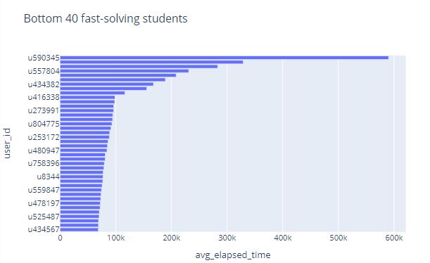

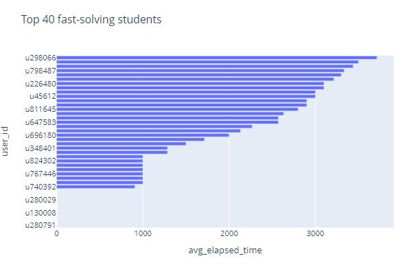We take the average time it takes students to do a question as an indicator of how fast students do it. These two figures respectively show the fastest and slowest students among the 5000 students, and the average time they spent doing the problems 

 

Note that some students spend very little time doing the questions, and the time is almost zero. We can almost judge that these students did not do the questions at all, and they chose blindly. We remove these students and rearrange them

bound=5000 # If the average time of doing the topic is less than 5000, it means that the student is most likely to be bad
ds=df.loc[:,['user_id','elapsed_time']].groupby('user_id').mean()
ds=ds.reset_index(drop=False)
ds.columns=['user_id','avg_elapsed_time']
bad_user_ids=ds[ds['avg_elapsed_time']<bound]['user_id'].to_list()
df_drop=df.drop(df[df['user_id'].isin(bad_user_ids)].index)
print('bad students number is ',len(bad_user_ids))
print('length of table after dropping is ',len(df_drop))

bad students number is  61
length of table after dropping is  567778

After dropping

ds=df_drop['user_id'].value_counts().reset_index(drop=False)
ds.columns=['user_id','count']
ds_tail=ds.sort_values(by=['count'],axis=0).tail(40)
fig_tail = px.bar(
    ds_tail,
    x = 'count',
    y = 'user_id',
    orientation='h',
    title='Top 40 active students after dropping some students'
)
fig_tail.show("svg")

This figure shows the 40 most active students after dropping some bad students.

ds=df_drop.loc[:,['user_id','elapsed_time']].groupby('user_id').mean()
ds=ds.reset_index(drop=False)
ds.columns=['user_id','avg_elapsed_time']

ds_head=ds.sort_values(by=['avg_elapsed_time'],axis=0).head(40)
fig_head = px.bar(
    ds_head,
    x = 'avg_elapsed_time',
    y = 'user_id',
    orientation='h',
    title='Top 40 fast-solving students after dropping some students'
)
fig_head.show("svg")

This figure respectively show the more reasonable fastest students among the 5000 students than before, and the average time they spent doing the problems.

Sort question_id

ds=df.loc[:,['question_id','elapsed_time']].groupby('question_id').mean()
ds=ds.reset_index(drop=False)
ds_tail=ds.sort_values(by=['elapsed_time'],axis=0).tail(40)
fig_tail = px.bar(
    ds_tail,
    x = 'elapsed_time',
    y = 'question_id',
    orientation='h',
    title='Top 40 question_id by the average of elapsed_time'
)
fig_tail.show("svg")
ds_head=ds.sort_values(by=['elapsed_time'],axis=0).head(40)
fig_head = px.bar(
    ds_head,
    x = 'elapsed_time',
    y = 'question_id',
    orientation='h',
    title='Bottom 40 question_id by the average of elapsed_time'
)
fig_head.show("svg")

 

 

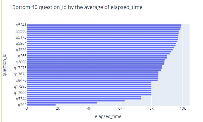
We can judge the difficulty of this question from the average time spent on a question.

These two figures reflect the difficulty of the questions and shows the ids of the 40 most difficult and 40 easiest questions.s

Appearence of Questions

ds=df['question_id'].value_counts().reset_index(drop=False)
ds.columns=['question_id','count']
ds_tail=ds.sort_values(by=['count'],axis=0).tail(40)
fig_tail = px.bar(
    ds_tail,
    x = 'count',
    y = 'question_id',
    orientation='h',
    title='Top 40 question_id by the number of appearance'
)
fig_tail.show("svg")
ds_head=ds.sort_values(by=['count'],axis=0).head(40)
fig_head = px.bar(
    ds_head,
    x = 'count',
    y = 'question_id',
    orientation='h',
    title='Bottom 40 question_id by the number of appearance'
)
fig_head.show("svg")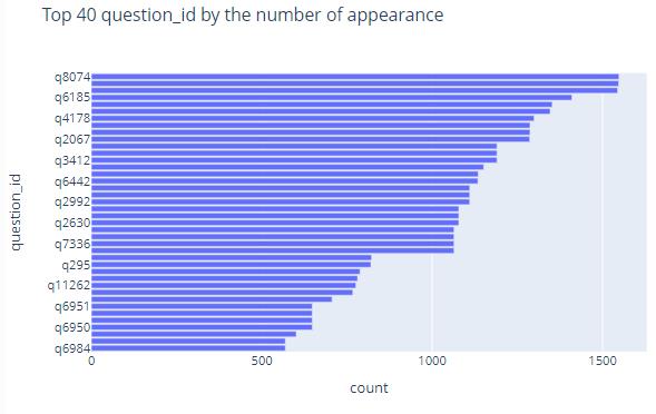

These two images reflect the 40 questions that were drawn the most frequently and the 40 questions that were drawn the least frequently

ds2=df['question_id'].value_counts().reset_index(drop=False)
ds2.columns=['question_id','count']
def convert_id2int(x):
    return pd.Series(map(lambda t:int(t[1:]),x))
ds2['question_id']=convert_id2int(ds2['question_id'])
ds2.sort_values(by=['question_id'])
fig = px.histogram(
    ds2,
    x = 'question_id',
    y = 'count',
    title='question distribution'
)
fig.show("svg")

Question’s Option Selected Most Frequently

ds=df.loc[:,['question_id','user_answer','user_id']].groupby(['question_id','user_answer']).count()

most_count_dict=
for id in df.question_id.unique():
    most_count=ds.loc[id].apply(lambda x:x.max())[0]
    most_count_dict[id]=most_count
ds2=ds.apply(lambda x:x-most_count_dict[x.name[0]],axis=1)
ds2=ds2[ds2.user_id==0]
ds2=ds2.reset_index(drop=False).loc[:,['question_id','user_answer']]
ds2.columns=['question_id','most_answer']
ds2.index=ds2['question_id']
ds2['most_answer']

question_id
q1        b
q10       d
q100      c
q1000     c
q10000    b
         ..
q9995     d
q9996     a
q9997     d
q9998     a
q9999     b
Name: most_answer, Length: 12215, dtype: object

This shows the most selected options (including not choose) for each question.

Note that if there are multiple options for a question to be selected most frequently, the table will also contain them.

Choices Distribution

ds = df['user_answer'].value_counts().reset_index(drop=False)
ds.columns = ['user_answer', 'percent']

ds['percent']=ds['percent']/len(df)
ds = ds.sort_values(by=['percent'])

fig = px.pie(
    ds,
    names = ds['user_answer'],
    values = 'percent',
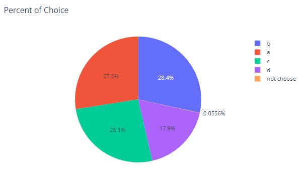
    title = 'Percent of Choice'
)

fig.show("svg")

We use a pie chart to show the distribution of the proportions of a, b, c, d and not choose among the options selected by the 5000 students.

Sort By Time Stamp

import time
import datetime
df_time=df.copy()
columns=df.columns.to_list()
columns[1]='time'
df_time.columns=columns
df_time['time'] /= 1000
df_time['time']=pd.Series(map(datetime.datetime.fromtimestamp,df_time['time']))
df_time

	user_id	time	solving_id	question_id	user_answer	elapsed_time
0	u717875	2019-08-09 14:27:07.449	1	q4862	d	45000
1	u717875	2019-08-09 14:27:37.492	2	q6747	d	24000
2	u717875	2019-08-09 14:28:05.743	3	q326	c	25000
3	u717875	2019-08-09 14:28:36.475	4	q6168	a	27000
4	u717875	2019-08-09 14:28:57.148	5	q847	a	17000
...	...	...	...	...	...	...
574251	u177603	2018-06-30 23:16:48.931	15	q6984	b	44250
574252	u177603	2018-06-30 23:23:17.614	16	q7335	c	95750
574253	u177603	2018-06-30 23:23:18.181	16	q7336	a	95750
574254	u177603	2018-06-30 23:23:18.879	16	q7337	c	95750
574255	u177603	2018-06-30 23:23:19.425	16	q7338	b	95750

574256 rows × 6 columns

This table shows the result of converting unix timestamp to datetime format

question distribution by time

ds_time_question=df_time.loc[:,['time','question_id']]
ds_time_question=ds_time_question.sort_values(by=['time'])
ds_time_question

	time	question_id
503014	2017-05-11 05:17:10.922	q129
503015	2017-05-11 05:17:34.561	q8058
503016	2017-05-11 05:17:56.806	q8120
503017	2017-05-11 05:18:22.591	q157
503018	2017-05-11 05:18:43.085	q52
...	...	...
108215	2019-12-03 00:48:27.437	q776
108216	2019-12-03 00:59:38.437	q10847
108217	2019-12-03 00:59:38.437	q10844
108218	2019-12-03 00:59:38.437	q10845
108219	2019-12-03 00:59:38.437	q10846

574256 rows × 2 columns

This table shows the given questions in chronological order.And we can see that the earliest question q127 is on May 11, 2017, and the latest question q10846 is on December 3, 2019.

ds_time_question['year']=pd.Series(map(lambda x :x.year,ds_time_question['time']))
ds_time_question['month']=pd.Series(map(lambda x :x.month,ds_time_question['time']))
ds=ds_time_question.loc[:,['year','month']].value_counts()

years=ds_time_question['year'].unique()
years.sort()
fig=make_subplots(
    rows=2,
    cols=2,
    start_cell='top-left',
    subplot_titles=tuple(map(str,years))
)
traces=[
    go.Bar(
        x=ds[year].reset_index().sort_values(by=['month'],axis=0)['month'].to_list(),
        y=ds[year].reset_index().sort_values(by=['month'],axis=0)[0].to_list(),
        name='Year: '+str(year),
        text=[ds[year][month] for month in ds[year].reset_index().sort_values(by=['month'],axis=0)['month'].to_list()],
        textposition='auto'
    ) for year in years
]
for i in range(len(traces)):
    fig.append_trace(traces[i],(i//2)+1,(i%2)+1)

fig.update_layout(title_text='Bar of the distribution of the number of question solved in  years'.format(len(traces)))
fig.show('svg')

 

1. These three figures show the distribution of the number of problems solved in each month of 2017, 2018, and 2019.

2. And the number of questions solved is gradually increasing.

3. And the number of questions solved in March, 4, May, and June is generally small.

user distribution by time

ds_time_user=df_time.loc[:,['user_id','time']]
ds_time_user=ds_time_user.sort_values(by=['time'])
ds_time_user

	user_id	time
503014	u21056	2017-05-11 05:17:10.922
503015	u21056	2017-05-11 05:17:34.561
503016	u21056	2017-05-11 05:17:56.806
503017	u21056	2017-05-11 05:18:22.591
503018	u21056	2017-05-11 05:18:43.085
...	...	...
108215	u9476	2019-12-03 00:48:27.437
108216	u9476	2019-12-03 00:59:38.437
108217	u9476	2019-12-03 00:59:38.437
108218	u9476	2019-12-03 00:59:38.437
108219	u9476	2019-12-03 00:59:38.437

574256 rows × 2 columns

This table shows the students who did the questions in order of time.And we can see that the first student who does the problem is u21056, and the last student who does the problem is u9476.

ds_time_user=df_time.loc[:,['user_id','time']]
ds_time_user=ds_time_user.sort_values(by=['time'])
ds_time_user['year']=pd.Series(map(lambda x :x.year,ds_time_user['time']))
ds_time_user['month']=pd.Series(map(lambda x :x.month,ds_time_user['time']))
ds_time_user.drop(['time'],axis=1,inplace=True)
ds=ds_time_user.groupby(['year','month']).nunique()

years=ds_time_user['year'].unique()
years.sort()
fig=make_subplots(
    rows=2,
    cols=2,
    start_cell='top-left',
    subplot_titles=tuple(map(str,years))
)
traces=[
    go.Bar(
        x=ds.loc[year].reset_index()['month'].to_list(),
        y=ds.loc[year].reset_index()['user_id'].to_list(),
        name='Year: '+str(year),
        text=[ds.loc[year].loc[month,'user_id'] for month in ds.loc[year].reset_index()['month'].to_list()],
        textposition='auto'
    ) for year in years
]
for i in range(len(traces)):
    fig.append_trace(traces[i],(i//2)+1,(i%2)+1)

fig.update_layout(title_text='Bar of the distribution of the number of active students in  years'.format(len(traces)))
fig.show('svg')

1. These three graphs respectively show the number of students active on the system in each month of 2017, 2018, and 2019.

2. And we can see that the number of active students in 2019 is generally more than that in 2018, and there are more in 2018 than in 2017, indicating that the number of users of the system is gradually increasing.

3. Note that the number of students is not repeated here