[读书笔记]机器学习:实用案例解析
Posted gy_jerry
tags:
篇首语:本文由小常识网(cha138.com)小编为大家整理,主要介绍了[读书笔记]机器学习:实用案例解析相关的知识,希望对你有一定的参考价值。
第4章 排序:智能收件箱
有监督学习与无监督学习:有监督学习已有明确的输出实例;无监督学习在开始处理数据时预先并没有已知的输出实例。
理论上邮件的优先级特征:
- 社交特征:收件人与发件人之间的交互程度
- 内容特征:收件人对邮件采取行为(回复、标记等)与某些特征词之间相关
- 线程特征:记录用户在当前线程下的交互行为
- 标签特征:检查用户通过过滤器给邮件赋予的标签(标记)
由于数据量不足,本文用于替代的优先级特征:(需要抽取的元素)
- 社交特征:来自某一发件人的邮件量(发件人地址)
- 时间量度:(接受时间日期)
- 线程特征:是否活跃(主题)
- 内容特征:高频词分析(邮件正文)
#machine learing for heckers
#chapter 4
library(tm)
library(ggplot2)
library(plyr)

easyham.path <- "ML_for_Hackers/03-Classification/data/easy_ham/"
###############################################
#抽取特征集合
###############################################
#输入邮件路径,返回特征信息
#把路径作为数据的最后一列保存,可以使测试阶段的排序更容易一些(书上这么写的,没看懂为什么)
parse.email <- function(path){
  full.msg <- msg.full(path)
  date <- get.date(full.msg)
  from <- get.from(full.msg)
  subj <- get.subject(full.msg)
  msg <- get.msg(full.msg)
  return(c(date, from, subj, msg, path))
}
#辅助函数的编写
#读取内容
#按行读取,每一行的内容对应向量中的一个元素
msg.full <- function(path){
  con <- file(path, open = "rt", encoding = "latin1")
  msg <- readLines(con)
  close(con)
  return(msg)
}
#正则表达式抽取信息
#抽取发件地址:
#两种格式:From: JM<j@xx.com>; From: j@xx.com(JM)
#grepl()以"From: "作为匹配条件,返回是(1)否(0)匹配;匹配的一行存入from中
#方括号创建字符集:冒号、尖括号、空格,作为拆分文本的标志,存入列表中的第一个元素
#将空元素过滤掉
#查找包含"@"字符的元素并返回
get.from <- function(msg.vec){
  from <- msg.vec[grepl("From: ", msg.vec)]
  from <- strsplit(from, \'[":<> ]\')[[1]]
  from <- from[which(from != "" & from != " ")]
  return(from[grepl("@", from)][1])
}
#抽取正文
get.msg <- function(msg.vec){
  msg <- msg.vec[seq(which(msg.vec == "")[1]+1, length(msg.vec), 1)]
  return(paste(msg, collapse = "\\n"))
}
#抽取主题
#正则匹配主题特征(有的邮件没有主题)
#如果长度大于0,返回第2个元素(第1个元素是"Subject")否则返回空字符
#如果不设条件,在grepl()一类函数得不到匹配时,会返回一个指定的值,
#如integer(0)或character(0)
get.subject <- function(msg.vec){
  subj <- msg.vec[grepl("Subject: ", msg.vec)]
  if(length(subj) > 0){
    return(strsplit(subj, "Subject: ")[[1]][2])
  }else{
    return("")
  }
}
#抽取日期
#需要解决的问题:
#1. 邮件头中会有许多行与"Date: "匹配,但是真正需要的是只有字符串首部出现的
#利用这一点,要求正则表达式只匹配在字符串首部的"Date: ",使用脱字符"^Date: "
#2. 有可能在正文中也匹配上,所以只需要保存第一次匹配成功的字符串即可
#3. 处理文本:拆分字符:加号或减号或冒号
#4. 将首部或者尾部的空白字符替换掉
#5. 只返回符合格式的部分,除掉25字符以后的内容
get.date <- function(msg.vec){
  date.grep <- grepl("^Date: ", msg.vec)
  date.grep <- which(date.grep == TRUE)
  date <- msg.vec[date.grep[1]]
  date <- strsplit(date, "\\\\+|\\\\-|: ")[[1]][2]
  date <- gsub("^\\\\s+|\\\\s+$", "", date)
  return(strtrim(date, 25))
}
#处理邮件
easyham.docs <- dir(easyham.path)
easyham.docs <- easyham.docs[which(easyham.docs != "cmds")]
easyham.parse <- lapply(easyham.docs,
function(p) parse.email(paste(easyham.path, p, sep = "")))
ehparse.matrix <- do.call(rbind, easyham.parse)
allparse.df <- data.frame(ehparse.matrix, stringsAsFactors = FALSE)
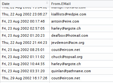
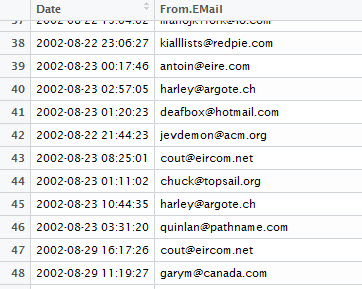
names(allparse.df) <- c("Date", "From.EMail", "Subject", "Message", "Path")
#时间格式不统一,需要进一步处理,转换为R中的POSIX对象,以便于排序
#将形如(Wed, 04 Dec 2002 11:36:32)和(04 Dec 2002 11:49:23)格式的字符串转换成POSIX格式
date.converter <- function(dates, pattern1, pattern2){
  pattern1.convert <- strptime(dates, pattern1)
  pattern2.convert <- strptime(dates, pattern2)
  pattern1.convert[is.na(pattern1.convert)] <- pattern2.convert[is.na(pattern2.convert)]
  return(pattern1.convert)
}
#指明需要转换的格式
pattern1 <- "%a, %d %b %Y %H:%M:%S"
pattern2 <- "%d %b %Y %H:%M:%S"
#系统区域设置,"LC_TIME"的设置会对as.POSIXlt()和strptime()的表现造成影响
#如果不进行设置,会使后面的处理后结果Date列全部缺失
Sys.setlocale("LC_TIME", "C")
allparse.df$Date <- date.converter(allparse.df$Date, pattern1, pattern2)
#转换成小写,统一格式
allparse.df$Subject <- tolower(allparse.df$Subject)
allparse.df$From.EMail <- tolower(allparse.df$From.EMail)
#根据时间排序 注意排序方法,使用with( , order()),虽然不直观,但是会经常用到,默认升序排列
#产生训练集:前一半作为训练集
priority.df <- allparse.df[with(allparse.df, order(Date)), ]
priority.train <- priority.df[1:(round(nrow(priority.df) / 2)), ]
######################################
#设置权重策略
######################################
#用ddply()在数据框上执行操作,对象是数据组From.EMail,summarise()创建了Freq保存频次信息
#日期一列会影响ddply()的操作,因此需要将该列删除或者是转成字符串类型,否则会出错
#直接应用书上的代码会提示如下error

#这里给出两种解决方案,都没问题
priority.train.temp1 <- priority.train[, c(2,3,4,5)]
priority.train.temp2 <- priority.train
priority.train.temp2$Date <- as.character(priority.train.temp2$Date)
from.weight <- ddply(priority.train.temp2, .(From.EMail), summarise, Freq = length(Subject))
#另外文件源码里给出另一种处理方式,得到的结果是一样的
library(reshape2)
from.weight <- melt(with(priority.train, table(From.EMail)), value.name="Freq")
#结果可视化
#排序、过滤频数小于6的观测、绘制图形
from.weight <- from.weight[with(from.weight, order(Freq)), ]
from.ex <- subset(from.weight, Freq > 6)
from.scales <- ggplot(from.ex) +
  geom_rect(aes(xmin = 1:nrow(from.ex) - 0.5,
                xmax = 1:nrow(from.ex) + 0.5,
                ymin = 0,
                ymax = Freq,
                fill = "lightgrey",
                color = "darkblue")) +
  scale_x_continuous(breaks = 1:nrow(from.ex), labels = from.ex$From.EMail) +
  coord_flip() +
  scale_fill_manual(values = c("lightgrey" = "lightgrey"), guide = "none") +
  scale_color_manual(values = c("darkblue" = "darkblue"), guide = "none") +
  ylab("Number of Emails Received (truncated at 6)") +
  xlab("Sender Address") +
  theme_bw() +
  theme(axis.text.y = element_text(size = 5, hjust = 1))
print(from.scales)
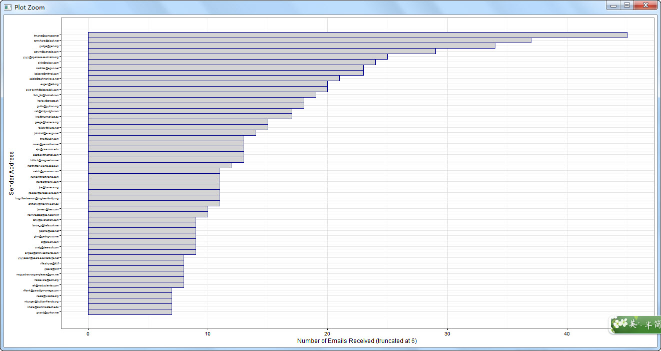
#根据条形图,只有几个人的数量很大,属于特殊情况,会导致权重偏移
#解决方案:尺度变换:不会因为极个别情况影响整体的阈值计算
#对数变换:观察绝对值权重、自然对数变换权重及常用对数变换权重
from.weight <- transform(from.weight,
                         Weight = log(Freq + 1),
                         log10Weight = log10(Freq + 1))
from.rescaled <- ggplot(from.weight, aes(x = 1:nrow(from.weight))) +
  geom_line(aes(y = Weight, linetype = "ln")) +
  geom_line(aes(y = log10Weight, linetype = "log10")) +
  geom_line(aes(y = Freq, linetype = "Absolute")) +
  scale_linetype_manual(values = c("ln" = 1,
                                   "log10" = 2,
                                   "Absolute" = 3),
                        name = "Scaling") +
  xlab("") +
  ylab("Number of emails Receieved") +
  theme_bw() +
  theme(axis.text.y = element_blank(), axis.text.x = element_blank())
print(from.rescaled)
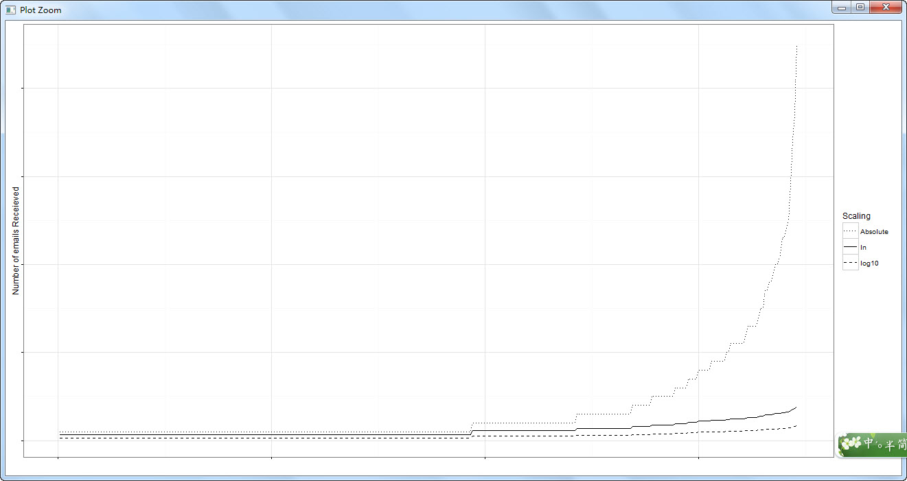
#绝对值权重过于陡峭,常用对数变换差异太弱,选择自然对数变换更加合理
#来自书中的警告:不允许特征集合中出现值为0的观测记录,否则log()会返回-Inf(负无穷),破坏整个结果
#线程活跃度的权重计算
#针对"re: "回复操作,可以找到相关线程
#返回所有带有"re: "的邮件的发件人和初始线程的主题
find.threads <- function(email.df){
  response.threads <- strsplit(email.df$Subject, "re: ")
  is.thread <- sapply(response.threads, function(subj) ifelse(subj[1] == "", TRUE, FALSE))
  threads <- response.threads[is.thread]
  senders <- email.df$From.EMail[is.thread]
  threads <- sapply(threads, function(t) paste(t[2:length(t)], collapse = "re: "))
  return(cbind(senders, threads))
}
threads.matrix <- find.threads(priority.train)
#根据线程中活跃的发件人赋予权重,增加在发件人上,但是只关注出现在threads.matrix中的发件人
#仍然采用自然对数变换的权重
email.thread <- function(threads.matrix){
  senders <- threads.matrix[, 1]
  senders.freq <- table(senders)
  senders.matrix <- cbind(names(senders.freq), senders.freq, log(senders.freq + 1))
  senders.df <- data.frame(senders.matrix, stringsAsFactors = FALSE)
  row.names(senders.df) <- 1:nrow(senders.df)
  names(senders.df) <- c("From.EMail", "Freq", "Weight")
  senders.df$Freq <- as.numeric(senders.df$Freq)
  senders.df$Weight <- as.numeric(senders.df$Weight)
  return(senders.df)
}
senders.df <- email.thread(threads.matrix)
#基于已知的活跃线程,追加权重:假设这个线程已知,用户会觉得这些更活跃的线程更重要
#unique()得到所有线程名称,thread.counts里存放了所有线程对应的活跃度及权重
#最后合并,返回线程名、频数、间隔时间和权重
get.threads <- function(threads.matrix, email.df){
  threads <- unique(threads.matrix[, 2])
  thread.counts <- lapply(threads,
                          function(t) thread.counts(t, email.df))
  thread.matrix <- do.call(rbind, thread.counts)
  return(cbind(threads, thread.matrix))
}
#输入线程主题和训练数据,通过所有邮件日期和时间戳,计算训练数据中这个线程接收了多少邮件
#thread.times找到了线程的时间戳,其向量长度就是该线程接收邮件的频数
#time.span是线程在训练数据中存在的时间:为了计算活跃度
#log.trans.weight是常用对数的权重
#一个线程中只有一条邮件记录的情况:训练数据开始收集数据时线程结束或训练数据结束收集时线程开始
#要剔除这种情况,返回缺失值
#实际情况中,频数小而间隔大,意味着trans.weight是远小于1的值,对它进行对数变换时,结果为负
#为了将权重计算不引入负值,进行仿射变换,即加10
thread.counts <- function(thread, email.df){
  thread.times <- email.df$Date[which(email.df$Subject == thread |
                                      email.df$Subject == paste("re:", thread))]
  freq <- length(thread.times)
  min.time <- min(thread.times)
  max.time <- max(thread.times)
  time.span <- as.numeric(difftime(max.time, min.time, units = "secs"))
  if(freq < 2){
    return(c(NA, NA, NA))
  }else{
    trans.weight <- freq / time.span
    log.trans.weight <- 10 + log(trans.weight, base = 10)
    return(c(freq, time.span, log.trans.weight))
  }
}
#生成权重数据,并做一定处理,最后用subset剔除缺失行
thread.weights <- get.threads(threads.matrix, priority.train)
thread.weights <- data.frame(thread.weights, stringsAsFactors = FALSE)
names(thread.weights) <- c("Thread", "Freq", "Response", "Weight")
thread.weights$Freq <- as.numeric(thread.weights$Freq)
thread.weights$Response <- as.numeric(thread.weights$Response)
thread.weights$Weight <- as.numeric(thread.weights$Weight)
thread.weights <- subset(thread.weights, is.na(thread.weights$Freq) == FALSE)
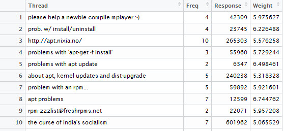
图中可以看到,即使有相同频数,因为响应时间不同,赋予的权重也不同。虽然对于一些人来说可能不会用这种方式排序,但是作为一种通用解决方案,需要这种量化的手段
#线程中的高频词权重:假设出现在活跃线程邮件主题中的高频词比低频词和出现在不活跃线程中的词项重要
#term.counts():输入词项向量和TDM选项列表,返回词项的TDM并抽取所有线程中的词项频次
term.counts <- function(term.vec, control){
  vec.corpus <- Corpus(VectorSource(term.vec))
  vec.tdm <- TermDocumentMatrix(vec.corpus, control = control)
  return(rowSums(as.matrix(vec.tdm)))
}
#计算词频,并只留下词项
#对词项进行赋予权重,该权重=该词项所在所有线程权重的平均值
#将向量转数据框,词项提取为名称,行名改为行号
thread.terms <- term.counts(thread.weights$Thread, control = list(stopwords = stopwords()))
thread.terms <- names(thread.terms)
term.weights <- sapply(thread.terms,
                        function(t) mean(thread.weights$Weight[grepl(t, thread.weights$Thread, fixed = TRUE)]))
term.weights <- data.frame(list(Term = names(term.weights), Weight = term.weights),
                            stringsAsFactors = FALSE, row.names = 1:length(term.weights))
#邮件词项权重:假设与已读邮件相似的邮件比完全陌生的邮件更重要
#计算出现在邮件中的词频,取对数变换值作为权重
#将负值权重剔除
msg.terms <- term.counts(priority.train$Message,
                         control = list(stopwords = stopwords(),
                                        removePunctuation = TRUE, removeNumbers = TRUE))
msg.weights <- data.frame(list(Term = names(msg.terms), Weight = log(msg.terms, base = 10)),
                          stringsAsFactors = FALSE, row.names = 1:length(msg.terms))
msg.weights <- subset(msg.weights, Weight > 0)
#################
#总结:共有5项权重数据框:
#from.weight(社交特征)
#senders.df(发件人在线程内的活跃度)
#thread.weights(线程的活跃度)
#term.weights(活跃线程的词项)
#msg.weights(所有邮件共有词项)
##############################################################
####################################
#训练和测试排序算法
####################################
#思路是给每封邮件都产生一个优先等级,这就要将前面提到的各个权重相乘
#因此需要对每封邮件都进行解析、抽取特征、匹配权重数据框并查找权重值
#用这些权重值的乘积作为排序的依据
####################
#首先执行权重查找,即主题和正文词项
#输入三个参数:待查找词项(字符串)、查找对象(权重数据框)、查找类型(T为词项,F为线程)
#返回权重值
#查找失败的情况:
#1.检查输入get.weights()的待查找词项长度是否大于0,如果输入无效则返回1不影响乘积运算
#2.match()对于没有匹配上的元素返回了NA,要将NA替换为1,通过判断match.weights为0即可
get.weights <- function(search.term, weight.df, term = TRUE){
  if(length(search.term) > 0 ){
    if(term){
      term.match <- match(names(search.term), weight.df$Term)
    }
    else{
      term.match <- match(search.term, weight.df$Thread)
    }
    match.weights <- weight.df$Weight[which(!is.na(term.match))]
    #书上的代码有误,但是表述正确
    if(length(match.weights) < 1){
      return(1)
    }
    else{
      return(mean(match.weights))
    }
  }
  else{
    return(1)
  }
}
#输入邮件路径,返回排序权重(rank)
rank.message <- function(path){
  #抽取四个特征:
  #msg[]1日期2发信人3主题4正文5路径
  msg <- parse.email(path)
  # Weighting based on message author

  # First is just on the total frequency
  #查找发件人地址权重,未匹配的返回1
  from <- ifelse(length(which(from.weight$From.EMail == msg[2])) > 0,
                 from.weight$Weight[which(from.weight$From.EMail == msg[2])], 1)

  # Second is based on senders in threads, and threads themselves
  #查找发件人活跃度权重,未匹配返回1
  thread.from <- ifelse(length(which(senders.df$From.EMail == msg[2])) > 0,
                        senders.df$Weight[which(senders.df$From.EMail == msg[2])], 1)
  #解析主题是否在线程内
  subj <- strsplit(tolower(msg[3]), "re: ")
  is.thread <- ifelse(subj[[1]][1] == "", TRUE, FALSE)
  #线程活跃度查找并匹配
  if(is.thread){
    activity <- get.weights(subj[[1]][2], thread.weights, term = FALSE)
  }
  else{
    activity <- 1
  }

  # Next, weight based on terms

  # Weight based on terms in threads
  #活跃线程词项权重匹配
  thread.terms <- term.counts(msg[3], control = list(stopwords = TRUE))
  thread.terms.weights <- get.weights(thread.terms, term.weights)

  # Weight based terms in all messages
  #正文词项权重匹配
  msg.terms <- term.counts(msg[4], control = list(stopwords = TRUE,  removePunctuation = TRUE,
                                                  removeNumbers = TRUE))
  msg.weights <- get.weights(msg.terms, msg.weights)

  # Calculate rank by interacting all weights
  #排序依据是所有查找到的权重的乘积
  rank <- prod(from, thread.from, activity, thread.terms.weights, msg.weights)
  #返回日期、发件人、主题、排序权重积
  return(c(msg[1], msg[2], msg[3], rank))
}
#启动排序算法
#按时间分为训练数据和测试数据,注意round()在处理.5的时候,返回的值是最靠近的偶数
train.paths <- priority.df$Path[1:(round(nrow(priority.df) / 2))]
test.paths <- priority.df$Path[((round(nrow(priority.df) / 2)) + 1):nrow(priority.df)]
#对训练数据进行处理,返回排序值
#警告可以忽略,应用suppressWarning()函数即可
train.ranks <- lapply(train.paths, rank.message)
train.ranks.matrix <- do.call(rbind, train.ranks)
train.ranks.matrix <- cbind(train.paths, train.ranks.matrix, "TRAINING")
train.ranks.df <- data.frame(train.ranks.matrix, stringsAsFactors = FALSE)
names(train.ranks.df) <- c("Message", "Date", "From", "Subj", "Rank", "Type")
train.ranks.df$Rank <- as.numeric(train.ranks.df$Rank)
#计算优先邮件的阈值(取中位数)新建列设置是否推荐
priority.threshold <- median(train.ranks.df$Rank)
train.ranks.df$Priority <- ifelse(train.ranks.df$Rank >= priority.threshold, 1, 0)
#将设定阈值的结果可视化:
threshold.plot <- ggplot(train.ranks.df, aes(x = Rank)) +
  stat_density(aes(fill="darkred")) +
  geom_vline(xintercept = priority.threshold, linetype = 2) +
  scale_fill_manual(values = c("darkred" = "darkred"), guide = "none") +
  theme_bw()
print(threshold.plot)
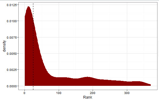
从图中可以看到阈值约为24,排序结果是明显的重尾分布,说明排序算法在训练集上表现不错
书中提到与标准差作为阈值,此时阈值为90. 中位数的做法有较大包容性,而标准差的方式将大部分邮件排除在外了
#测试集测试效果
test.ranks <- suppressWarnings(lapply(test.paths,rank.message))
test.ranks.matrix <- do.call(rbind, test.ranks)
test.ranks.matrix <- cbind(test.paths, test.ranks.matrix, "TESTING")
test.ranks.df <- data.frame(test.ranks.matrix, stringsAsFactors = FALSE)
names(test.ranks.df) <- c("Message","Date","From","Subj","Rank","Type")
test.ranks.df$Rank <- as.numeric(test.ranks.df$Rank)
test.ranks.df$Priority <- ifelse(test.ranks.df$Rank >= priority.threshold, 1, 0)
#合并训练集和测试集
final.df <- rbind(train.ranks.df, test.ranks.df)
Sys.setlocale("LC_TIME", "C")
final.df$Date <- date.converter(final.df$Date, pattern1, pattern2)
final.df <- final.df[rev(with(final.df, order(Date))), ]
在上图的基础上叠加测试数据的排序密度
testing.plot <- ggplot(subset(final.df, Type == "TRAINING"), aes(x = Rank)) +
  stat_density(aes(fill = Type, alpha = 0.65)) +
  stat_density(data = subset(final.df, Type == "TESTING"),
               aes(fill = Type, alpha = 0.65)) +
  geom_vline(xintercept = priority.threshold, linetype = 2) +
  scale_alpha(guide = "none") +
  scale_fill_manual(values = c("TRAINING" = "darkred", "TESTING" = "darkblue")) +
  theme_bw()
print(testing.plot)
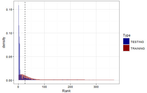
图表分析:
测试数据的分布尾部密度更高,说明更多邮件的优先级排序值不高;
密度估计不平滑,说明测试数据中包含了较多训练数据中没有出现的特征。
测试数据中排序在前面的邮件:
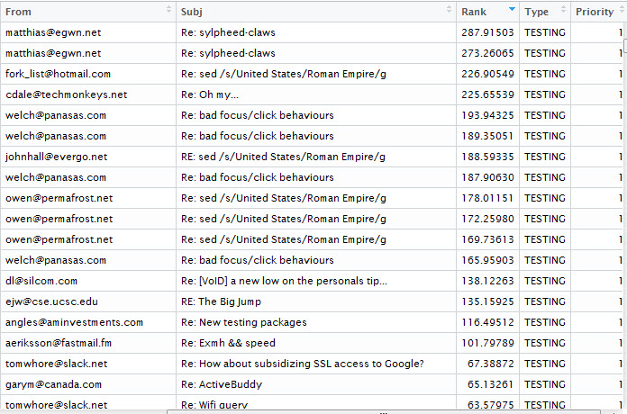
可以看到,该排序算法在线程上的表现较好,即相同线程的各个邮件大致在同一组;相同主题不同发件人也有不同的优先级。
以上是关于[读书笔记]机器学习:实用案例解析的主要内容,如果未能解决你的问题,请参考以下文章