coursera机器学习公开课笔记15: anomaly-detection

Posted 2020-11-04 snaildove

Note

This personal note is written after studying the opening course on the coursera website, Machine Learning by Andrew NG . And images, audios of this note all comes from the opening course.

01_density-estimation

In this next set of videos, I‘d like to tell you about a problem called Anomaly Detection. This is a reasonably commonly use you type machine learning. And one of the interesting aspects is that it‘s mainly for unsupervised problem, that there‘s some aspects of it that are also very similar to sort of the supervised learning problem. So, what is anomaly detection?

example

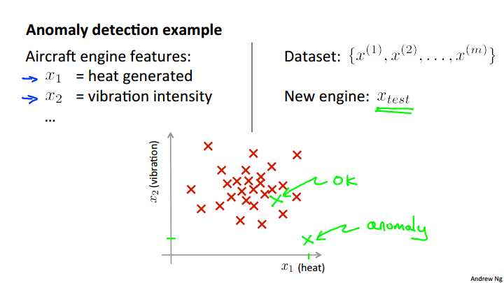
To explain it. Let me use the motivating example of: Imagine that you‘re a manufacturer of aircraft engines, and let‘s say that as your aircraft engines roll off the assembly line, you‘re doing, you know, QA or quality assurance testing, and as part of that testing you measure features of your aircraft engine, like maybe, you measure the heat generated, things like the vibrations and so on. I share some friends that worked on this problem a long time ago, and these were actually the sorts of features that they were collecting off actual aircraft engines so you now have a data set of X1 through Xm, if you have manufactured m aircraft engines, and if you plot your data, maybe it looks like this. So, each point here, each cross here as one of your unlabeled examples. So, the anomaly detection problem is the following. Let‘s say that on, you know, the next day, you have a new aircraft engine that rolls off the assembly line and your new aircraft engine has some set of features x-test. What the anomaly detection problem is, we want to know if this aircraft engine is anomalous in any way, in other words, we want to know if, maybe, this engine should undergo further testing because, or if it looks like an okay engine, and so it‘s okay to just ship it to a customer without further testing. So, if your new aircraft engine looks like a point over there, well, you know, that looks a lot like the aircraft engines we‘ve seen before, and so maybe we‘ll say that it looks okay. Whereas, if your new aircraft engine, if x-test, you know, were a point that were out here, so that if X1 and X2 are the features of this new example. If x-tests were all the way out there, then we would call that an anomaly. and maybe send that aircraft engine for further testing before we ship it to a customer, since it looks very different than the rest of the aircraft engines we‘ve seen before.

Desity estimation

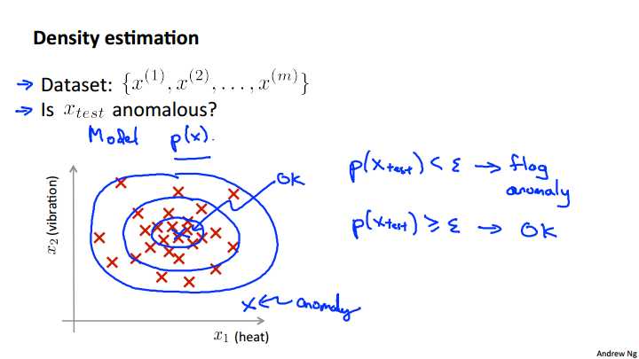
More formally in the anomaly detection problem, we‘re give some data sets, x1 through Xm of examples, and we usually assume that these end examples are normal or non-anomalous examples, and we want an algorithm to tell us if some new example x-test is anomalous. The approach that we‘re going to take is that given this training set, given the unlabeled training set, we‘re going to build a model for p of x. In other words, we‘re going to build a model for the probability of x, where x are these features of, say, aircraft engines. And so, having built a model of the probability of x we‘re then going to say that for the new aircraft engine, if p of x-test is less than some epsilon then we flag this as an anomaly. So we see a new engine that, you know, has very low probability under a model p of x that we estimate from the data, then we flag this anomaly, whereas if p of x-test is, say, greater than or equal to some small threshold. Then we say that, you know, okay, it looks okay. And so, given the training set, like that plotted here, if you build a model, hopefully you will find that aircraft engines, or hopefully the model p of x will say that points that lie, you know, somewhere in the middle, that‘s pretty high probability, whereas points a little bit further out have lower probability. Points that are even further out have somewhat lower probability, and the point that‘s way out here, the point that‘s way out there, would be an anomaly. Whereas the point that‘s way in there, right in the middle, this would be okay because p of x right in the middle of that would be very high cause we‘ve seen a lot of points in that region.

Here are some examples of applications of anomaly detection. Perhaps the most common application of anomaly detection is actually for detection if you have many users, and if each of your users take different activities, you know maybe on your website or in the physical plant or something, you can compute features of the different users activities. And what you can do is build a model to say, you know, what is the probability of different users behaving different ways. What is the probability of a particular vector of features of a users behavior so you know examples of features of a users activity may be on the website it‘d be things like, maybe x1 is how often does this user log in, x2, you know, maybe the number of what pages visited, or the number of transactions, maybe x3 is, you know, the number of posts of the users on the forum, feature x4 could be what is the typing speed of the user and some websites can actually track that was the typing speed of this user in characters per second. And so you can model p of x based on this sort of data. And finally having your model p of x, you can try to identify users that are behaving very strangely on your website by checking which ones have probably effects less than epsilon and maybe send the profiles of those users for further review. Or demand additional identification from those users, or some such to guard against you know, strange behavior or fraudulent behavior on your website. This sort of technique will tend of flag the users that are behaving unusually, not just users that maybe behaving fraudulently. So not just constantly having stolen or users that are trying to do funny things, or just find unusual users. But this is actually the technique that is used by many online websites that sell things to try identify users behaving strangely that might be indicative of either fraudulent behavior or of computer accounts that have been stolen. Another example of anomaly detection is manufacturing. So, already talked about the aircraft engine thing where you can find unusual, say, aircraft engines and send those for further review. A third application would be monitoring computers in a data center. I actually have some friends who work on this too. So if you have a lot of machines in a computer cluster or in a data center, we can do things like compute features at each machine. So maybe some features capturing you know, how much memory used, number of disc accesses, CPU load. As well as more complex features like what is the CPU load on this machine divided by the amount of network traffic on this machine? Then given the dataset of how your computers in your data center usually behave, you can model the probability of x, so you can model the probability of these machines having different amounts of memory use or probability of these machines having different numbers of disc accesses or different CPU loads and so on. And if you ever have a machine whose probability of x, p of x, is very small then you know that machine is behaving unusually and maybe that machine is about to go down, and you can flag that for review by a system administrator. And this is actually being used today by various data centers to watch out for unusual things happening on their machines. So, that‘s anomaly detection. In the next video, I‘ll talk a bit about the Gaussian distribution and review properties of the Gaussian probability distribution, and in videos after that, we will apply it to develop an anomaly detection algorithm.

summary

Problem Motivation
Just like in other learning problems, we are given a dataset \\({x^{(1)}, x^{(2)},\\dots,x^{(m)}}\\).
We are then given a new example, \\(x_{test}\\), and we want to know whether this new example is abnormal/anomalous.
We define a "model" \\(p(x)\\) that tells us the probability the example is not anomalous. We also use a threshold \\(?\\) (epsilon) as a dividing line so we can say which examples are anomalous and which are not.
A very common application of anomaly detection is detecting fraud:

• \\(x^{(i)} =\\) features of user i‘s activities
• Model \\(p(x)\\) from the data.
• Identify unusual users by checking which have \\(p(x)<?\\).

If our anomaly detector is flagging too many anomalous examples, then we need to decrease our threshold \\(?\\)

02_gaussian-distribution

In this video, I‘d like to talk about
the Gaussian distribution which is also called the normal distribution. In case you‘re already intimately familiar with the Gaussian distribution, it‘s probably okay to skip this video,but if you‘re not sure or if it has been a while since you‘ve worked with the Gaussian distribution or normal distribution then please do watch this video all the way to the end. And in the video after this we‘ll start applying the Gaussian distribution to developing an anomaly detection algorithm.

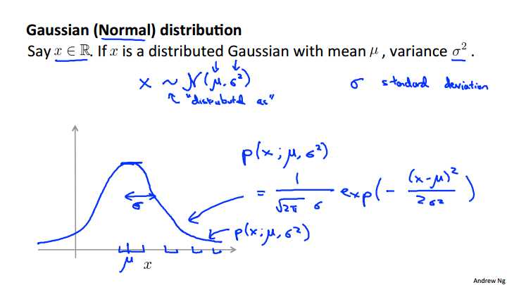
Let‘s say x is a row value‘s random variable, so x is a row number. If the probability distribution of x is Gaussian with mean mu and variance sigma squared. Then, we‘ll write this as x, the random variable. Tilde, this little tilde, this is distributed as. And then to denote a Gaussian distribution, sometimes I‘m going to write script N parentheses mu comma sigma script. So this script N stands for normal since Gaussian and normal they mean the thing are synonyms. And the Gaussian distribution is parametarized by two parameters, by a mean parameter which we denote mu and a variance parameter which we denote via sigma squared. If we plot the Gaussian distribution or Gaussian probability density. It‘ll look like the bell shaped curve which you may have seen before. And so this bell shaped curve is paramafied by those two parameters, mu and sequel. And the location of the center of this bell shaped curve is the mean mu. And the width of this bell shaped curve, roughly that, is this parameter, sigma, is also called one standard deviation, and so this specifies the probability of x taking on different values. So, x taking on values here in the middle here it‘s pretty high, since the Gaussian density here is pretty high, whereas x taking on values further, and further away will be diminishing in probability. Finally just for completeness let me write out the formula for the Gaussian distribution. So the probability of x, and I‘ll sometimes write this as the p (x) when we write this as P ( x ; mu, sigma squared), and so this denotes that the probability of X is parameterized by the two parameters mu and sigma squared. And the formula for the Gaussian density is this 1/ root 2 pi, sigma e (-(x-mu/g) squared/2 sigma squared. So there‘s no need to memorize this formula. This is just the formula for the bell-shaped curve over here on the left. There‘s no need to memorize it, and if you ever need to use this, you can always look this up. And so that figure on the left, that is what you get if you take a fixed value of mu and take a fixed value of sigma, and you plot P(x) so this curve here. This is really p(x) plotted as a function of X for a fixed value of Mu and of sigma squared. And by the way sometimes it‘s easier to think in terms of sigma squared that‘s called the variance. And sometimes is easier to think in terms of sigma. So sigma is called the standard deviation, and so it specifies the width of this Gaussian probability density, where as the square sigma, or sigma squared, is called the variance.

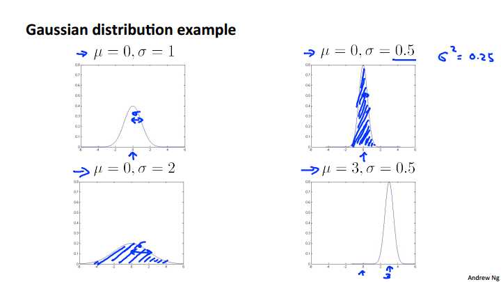
Let‘s look at some examples of what the Gaussian distribution looks like. If mu equals zero, sigma equals one. Then we have a Gaussian distribution that‘s centered around zero, because that‘s mu and the width of this Gaussian, so that‘s one standard deviation is sigma over there. Let‘s look at some examples of Gaussians. If mu is equal to zero and sigma equals one, then that corresponds to a Gaussian distribution that is centered at zero, since mu is zero, and the width of this Gaussian is is controlled by sigma by that variance parameter sigma. Here‘s another example. That same mu is equal to 0 and sigma is equal to .5 so the standard deviation is .5 and the variance sigma squared would therefore be the square of 0.5 would be 0.25 and in that case the Gaussian distribution, the Gaussian probability density goes like this. Is also sent as zero. But now the width of this is much smaller because the smaller the area is, the width of this Gaussian density is roughly half as wide. But because this is a probability distribution, the area under the curve, that‘s the shaded area there. That area must integrate to one this is a property of probability distributing. So this is a much taller Gaussian density because this half is Y but half the standard deviation but it twice as tall. Another example is sigma is equal to 2 then you get a much fatter a much wider Gaussian density and so here the sigma parameter controls that Gaussian distribution has a wider width. And once again, the area under the curve, that is the shaded area, will always integrate to one, that‘s the property of probability distributions and because it‘s wider it‘s also half as tall in order to still integrate to the same thing. And finally one last example would be if we now change the mu parameters as well. Then instead of being centered at 0 we now have a Gaussian distribution that‘s centered at 3 because this shifts over the entire Gaussian distribution.

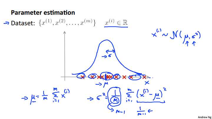
Next, let‘s talk about the Parameter estimation problem. So what‘s the parameter estimation problem? Let‘s say we have a dataset of m examples so exponents x m and lets say each of this example is a row number. Here in the figure I‘ve plotted an example of the dataset so the horizontal axis is the x axis and either will have a range of examples of x, and I‘ve just plotted them on this figure here. And the parameter estimation problem is, let‘s say I suspect that these examples came from a Gaussian distribution. So let‘s say I suspect that each of my examples, x i, was distributed. That‘s what this tilde thing means. Let‘s not suspect that each of these examples were distributed according to a normal distribution, or Gaussian distribution, with some parameter mu and some parameter sigma square. But I don‘t know what the values of these parameters are. The problem of parameter estimation is, given my data set, I want to try to figure out, well I want to estimate what are the values of mu and sigma squared. So if you‘re given a data set like this, it looks like maybe if I estimate what Gaussian distribution the data came from, maybe that might be roughly the Gaussian distribution it came from. With mu being the center of the distribution, sigma standing for the deviation controlling the width of this Gaussian distribution. Seems like a reasonable fit to the data. Because, you know, looks like the data has a very high probability of being in the central region, and a low probability of being further out, even though probability of being further out, and so on. So maybe this is a reasonable estimate of mu and sigma squared. That is, if it corresponds to a Gaussian distribution function that looks like this. So what I‘m going to do is just write out the formula the standard formulas for estimating the parameters Mu and sigma squared. Our estimate or the way we‘re going to estimate mu is going to be just the average of my example. So mu is the mean parameter. Just take my training set, take my m examples and average them. And that just means the center of this distribution. How about sigma squared? Well, the variance, I‘ll just write out the standard formula again, I‘m going to estimate as sum over one through m of x i minus mu squared. And so this mu here is actually the mu that I compute over here using this formula. And what the variance is, or one interpretation of the variance is that if you look at this term, that‘s the square difference between the value I got in my example minus the mean. Minus the center, minus the mean of the distribution. And so in the variance I‘m gonna estimate as just the average of the square differences between my examples, minus the mean. And as a side comment, only for those of you that are experts in statistics. If you‘re an expert in statistics, and if you‘ve heard of maximum likelihood estimation, then these parameters, these estimates, are actually the maximum likelihood estimates of the parameters of mu and sigma squared but if you haven‘t heard of that before don‘t worry about it, all you need to know is that these are the two standard formulas for how to figure out what are mu and Sigma squared given the data set. Finally one last side comment again only for those of you that have maybe taken the statistics class before but if you‘ve taken statistics This class before. Some of you may have seen the formula here where this is M-1 instead of M so this first term becomes 1/M-1 instead of 1/M. In machine learning people tend to learn 1/M formula but in practice whether it is 1/M or 1/M-1 it makes essentially no difference assuming M is reasonably large. a reasonably large training set size. So just in case you‘ve seen this other version before. In either version it works just about equally well but in machine learning most people tend to use 1/M in this formula.And the two versions have slightly different theoretical properties like these are different math properties. Bit of practice it really makes makes very little difference, if any.

So, hopefully you now have a good sense of what the Gaussian distribution looks like, as well as how to estimate the parameters mu and sigma squared of Gaussian distribution if you‘re given a training set, that is if you‘re given a set of data that you suspect comes from a Gaussian distribution with unknown parameters, mu and sigma squared. In the next video, we‘ll start to take this and apply it to develop an anomaly detection algorithm.

summary

The Gaussian Distribution is a familiar bell-shaped curve that can be described by a function \\(\\mathcal{N}(\\mu,\\sigma^2)\\)
Let x∈?. If the probability distribution of x is Gaussian with mean μ, variance \\(\\sigma^2\\), then:
\\[x \\sim \\mathcal{N}(\\mu, \\sigma^2)\\]
The little ～ or ‘tilde‘ can be read as "distributed as."
The Gaussian Distribution is parameterized by a mean and a variance.
Mu, or μ, describes the center of the curve, called the mean. The width of the curve is described by sigma, or σ, called the standard deviation.
The full function is as follows:
\\[\\large p(x;\\mu,\\sigma^2) = \\dfrac{1}{\\sigma\\sqrt{(2\\pi)}}e^{-\\dfrac{1}{2}(\\dfrac{x - \\mu}{\\sigma})^2}\\]
We can estimate the parameter μ from a given dataset by simply taking the average of all the examples:
\\[\\mu = \\dfrac{1}{m}\\displaystyle \\sum_{i=1}^m x^{(i)}\\]
We can estimate the other parameter, \\(\\sigma^2\\), with our familiar squared error formula:
\\[\\sigma^2 = \\dfrac{1}{m}\\displaystyle \\sum_{i=1}^m(x^{(i)} - \\mu)^2\\]

03_algorithm

In the last video, we talked about the Gaussian distribution. In this video lets apply that to develop an anomaly detection algorithm.

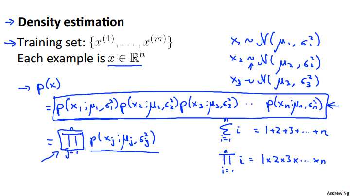
Let‘s say that we have an unlabeled training set of M examples, and each of these examples is going to be a feature in Rn so your training set could be, feature vectors from the last M aircraft engines being manufactured. Or it could be features from m users or something else. The way we are going to address anomaly detection, is we are going to model p of x from the data sets. We‘re going to try to figure out what are high probability features, what are lower probability types of features. So, x is a vector and what we are going to do is model p of x, as probability of x1, that is of the first component of x, times the probability of x2, that is the probability of the second feature, times the probability of the third feature, and so on up to the probability of the final feature of Xn. Now I‘m leaving space here cause I‘ll fill in something in a minute. So, how do we model each of these terms, p of X1, p of X2, and so on. What we‘re going to do, is assume that the feature, X1, is distributed according to a Gaussian distribution, with some mean, which you want to write as mu1 and some variance, which I‘m going to write as sigma squared 1, and so p of X1 is going to be a Gaussian probability distribution, with mean mu1 and variance sigma squared 1. And similarly I‘m going to assume that X2 is distributed, Gaussian, that‘s what this little tilda stands for, that means distributed Gaussian with mean mu2 and Sigma squared 2, so it‘s distributed according to a different Gaussian, which has a different set of parameters, mu2 sigma square 2. And similarly, you know, X3 is yet another Gaussian, so this can have a different mean and a different standard deviation than the other features, and so on, up to XN. And so that‘s my model. Just as a side comment for those of you that are experts in statistics, it turns out that this equation that I just wrote out actually corresponds to an independence assumption on the values of the features x1 through xn. But in practice it turns out that the algorithm of this fragment, it works just fine, whether or not these features are anywhere close to independent and even if independence assumption doesn‘t hold true this algorithm works just fine. But in case you don‘t know those terms I just used independence assumptions and so on, don‘t worry about it. You‘ll be able to understand it and implement this algorithm just fine and that comment was really meant only for the experts in statistics.

Finally, in order to wrap this up, let me take this expression and write it a little bit more compactly. So, we‘re going to write this is a product from J equals one through N, of P of XJ parameterized by mu j comma sigma squared j. So this funny symbol here, there is capital Greek alphabet pi, that funny symbol there corresponds to taking the product of a set of values. And so, you‘re familiar with the summation notation, so the sum from i equals one through n, of i. This means 1 + 2 + 3 plus dot dot dot, up to n. Where as this funny symbol here, this product symbol, right product from i equals 1 through n of i. Then this means that, it‘s just like summation except that we‘re now multiplying. This becomes 1 times 2 times 3 times up to N. And so using this product notation, this product from j equals 1 through n of this expression. It‘s just more compact, it‘s just shorter way for writing out this product of of all of these terms up there. Since we‘re are taking these p of x j given mu j comma sigma squared j terms and multiplying them together. And, by the way the problem of estimating this distribution p of x, they‘re sometimes called the problem of density estimation. Hence the title of the slide.

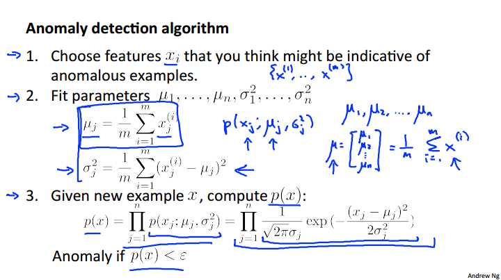
So putting everything together, here is our anomaly detection algorithm. The first step is to choose features, or come up with features xi that we think might be indicative of anomalous examples. So what I mean by that, is, try to come up with features, so that when there‘s an unusual user in your system that may be doing fraudulent things, or when the aircraft engine examples, you know there‘s something funny, something strange about one of the aircraft engines. Choose features X I, that you think might take on unusually large values, or unusually small values, for what an anomalous example might look like. But more generally, just try to choose features that describe general properties of the things that you‘re collecting data on. Next, given a training set, of M, unlabled examples, X1 through X M, we then fit the parameters, mu 1 through mu n, and sigma squared 1 through sigma squared n, and so these were the formulas similar to the formulas we have in the previous video, that we‘re going to use the estimate each of these parameters, and just to give some interpretation, mu J, that‘s my average value of the j feature. Mu j goes in this term p of xj. which is parametrized by mu J and sigma squared J. And so this says for the mu J just take the mean over my training set of the values of the j feature. And, just to mention, that you do this, you compute these formulas for j equals one through n. So use these formulas to estimate mu 1, to estimate mu 2, and so on up to mu n, and similarly for sigma squared, and it‘s also possible to come up with vectorized versions of these. So if you think of mu as a vector, so mu if is a vector there‘s mu 1, mu 2, down to mu n, then a vectorized version of that set of parameters can be written like so sum from 1 equals one through n xi. So, this formula that I just wrote out estimates this xi as the feature vectors that estimates mu for all the values of n simultaneously. And it‘s also possible to come up with a vectorized formula for estimating sigma squared j. Finally, when you‘re given a new example, so when you have a new aircraft engine and you want to know is this aircraft engine anomalous. What we need to do is then compute p of x, what‘s the probability of this new example? So, p of x is equal to this product, and what you implement, what you compute, is this formula and where over here, this thing here this is just the formula for the Gaussian probability, so you compute this thing, and finally if this probability is very small, then you flag this thing as an anomaly. Here‘s an example of an application of this method. Let‘s say we have this data set plotted on the upper left of this slide. if you look at this, well, lets look the feature of x1. If you look at this data set, it looks like on average, the features x1 has a mean of about 5 and the standard deviation, if you only look at just the x1 values of this data set has the standard deviation of maybe 2. So that sigma 1 and looks like x2 the values of the features as measured on the vertical axis, looks like it has an average value of about 3, and a standard deviation of about 1. So if you take this data set and if you estimate mu1, mu2, sigma1, sigma2, this is what you get. And again, I‘m writing sigma here, I‘m think about standard deviations, but the formula on the previous 5 actually gave the estimates of the squares of theses things, so sigma squared 1 and sigma squared 2. So, just be careful whether you are using sigma 1, sigma 2, or sigma squared 1 or sigma squared 2. So, sigma squared 1 of course would be equal to 4, for example, as the square of 2. And in pictures what p of x1 parametrized by mu1 and sigma squared 1 and p of x2, parametrized by mu 2 and sigma squared 2, that would look like these two distributions over here. And, turns out that if were to plot of p of x, right, which is the product of these two things, you can actually get a surface plot that looks like this. This is a plot of p of x, where the height above of this, where the height of this surface at a particular point, so given a particular x1 x2 values of x2 if x1 equals 2, x equal 2, that‘s this point. And the height of this 3-D surface here, that‘s p of x. So p of x, that is the height of this plot, is literally just p of x1 parametrized by mu 1 sigma squared 1, times p of x2 parametrized by mu 2 sigma squared 2. Now, so this is how we fit the parameters to this data. Let‘s see if we have a couple of new examples. Maybe I have a new example there. Is this an anomaly or not? Or, maybe I have a different example, maybe I have a different second example over there. So, is that an anomaly or not? They way we do that is, we would set some value for Epsilon, let‘s say I‘ve chosen Epsilon equals 0.02. I‘ll say later how we choose Epsilon. But let‘s take this first example, let me call this example X1 test. And let me call the second example X2 test. What we do is, we then compute p of X1 test, so we use this formula to compute it and this looks like a pretty large value. In particular, this is greater than, or greater than or equal to epsilon. And so this is a pretty high probability at least bigger than epsilon, so we‘ll say that X1 test is not an anomaly. Whereas, if you compute p of X2 test, well that is just a much smaller value. So this is less than epsilon and so we‘ll say that that is indeed an anomaly, because it is much smaller than that epsilon that we then chose. And in fact, I‘d improve it here. What this is really saying is that, you look through the 3d surface plot. It‘s saying that all the values of x1 and x2 that have a high height above the surface, corresponds to an a non-anomalous example of an OK or normal example. Whereas all the points far out here, all the points out here, all of those points have very low probability, so we are going to flag those points as anomalous, and so it‘s gonna define some region, that maybe looks like this, so that everything outside this, it flags as anomalous, whereas the things inside this ellipse I just drew, if it considers okay, or non-anomalous, not anomalous examples. And so this example x2 test lies outside that region, and so it has very small probability, and so we consider it an anomalous example.

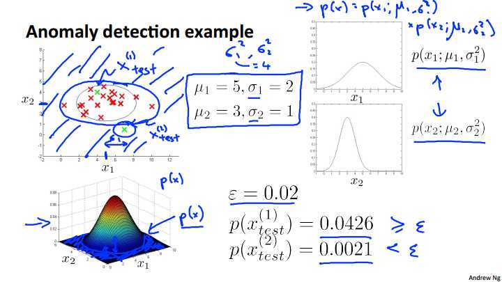
In this video we talked about how to estimate p of x, the probability of x, for the purpose of developing an anomaly detection algorithm. And in this video, we also stepped through an entire process of giving data set, we have, fitting the parameters, doing parameter estimations. We get mu and sigma parameters, and then taking new examples and deciding if the new examples are anomalous or not. In the next few videos we will delve deeper into this algorithm, and talk a bit more about how to actually get this to work well.

summary

Given a training set of examples, \\(\\lbrace x^{(1)},\\dots,x^{(m)}\\rbrace\\) where each example is a vector, \\(x \\in \\mathbb{R}^n\\).
\\[p(x) = p(x_1;\\mu_1,\\sigma_1^2)p(x_2;\\mu_2,\\sigma^2_2)\\cdots p(x_n;\\mu_n,\\sigma^2_n)\\]
In statistics, this is called an "independence assumption" on the values of the features inside training example x.
More compactly, the above expression can be written as follows:
\\[= \\displaystyle \\prod^n_{j=1} p(x_j;\\mu_j,\\sigma_j^2)\\]
The algorithm
Choose features \\(x_i\\) that you think might be indicative of anomalous examples.
Fit parameters \\[\\mu_1,\\dots,\\mu_n,\\sigma_1^2,\\dots,\\sigma_n^2\\]
Calculate \\(\\mu_j = \\dfrac{1}{m}\\displaystyle \\sum_{i=1}^m x_j^{(i)}\\)
Calculate \\(\\sigma^2_j = \\dfrac{1}{m}\\displaystyle \\sum_{i=1}^m(x_j^{(i)} - \\mu_j)^2\\)
Given a new example x, compute p(x):
\\[p(x) = \\displaystyle \\prod^n_{j=1} p(x_j;\\mu_j,\\sigma_j^2) = \\prod\\limits^n_{j=1} \\dfrac{1}{\\sqrt{2\\pi}\\sigma_j}exp(-\\dfrac{(x_j - \\mu_j)^2}{2\\sigma^2_j})\\]
Anomaly if p(x)<?
A vectorized version of the calculation for μ is \\(\\mu = \\dfrac{1}{m}\\displaystyle \\sum_{i=1}^m x^{(i)}\\). You can vectorize \\(\\sigma^2\\) similarly.

02_building-an-anomaly-detection-system

01_developing-and-evaluating-an-anomaly-detection-system

In the last video, we developed an anomaly detection algorithm. In this video, I like to talk about the process of how to go about developing a specific application of anomaly detection to a problem and in particular this will focus on the problem of how to evaluate an anomaly detection algorithm.

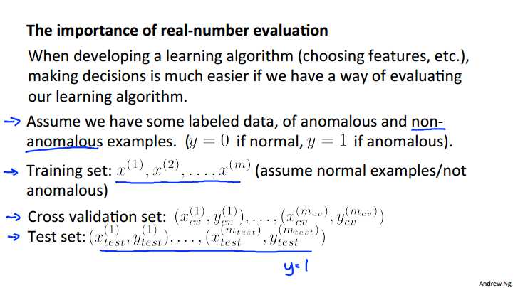
In previous videos, we‘ve already talked about the importance of real number evaluation and this captures the idea that when you‘re trying to develop a learning algorithm for a specific application, you need to often make a lot of choices like, you know, choosing what features to use and then so on. And making decisions about all of these choices is often much easier, and if you have a way to evaluate your learning algorithm that just gives you back a number. So if you‘re trying to decide, you know, I have an idea for one extra feature, do I include this feature or not. If you can run the algorithm with the feature, and run the algorithm without the feature, and just get back a number that tells you, you know, did it improve or worsen performance to add this feature? Then it gives you a much better way, a much simpler way, with which to decide whether or not to include that feature. So in order to be able to develop an anomaly detection system quickly, it would be a really helpful to have a way of evaluating an anomaly detection system. In order to do this, in order to evaluate an anomaly detection system, we‘re actually going to assume have some labeled data. So, so far, we‘ll be treating anomaly detection as an unsupervised learning problem, using unlabeled data. But if you have some labeled data that specifies what are some anomalous examples, and what are some non-anomalous examples, then this is how we actually think of as the standard way of evaluating an anomaly detection algorithm. So taking the aircraft engine example again. Let‘s say that, you know, we have some label data of just a few anomalous examples of some aircraft engines that were manufactured in the past that turns out to be anomalous. Turned out to be flawed or strange in some way. Let‘s say we use we also have some non-anomalous examples, so some perfectly okay examples. I‘m going to use y equals 0 to denote the normal or the non-anomalous example and y equals 1 to denote the anomalous examples. The process of developing and evaluating an anomaly detection algorithm is as follows. We‘re going to think of it as a training set and talk about the cross validation in test sets later, but the training set we usually think of this as still the unlabeled training set. And so this is our large collection of normal, non-anomalous or not anomalous examples. And usually we think of this as being as non-anomalous, but it‘s actually okay even if a few anomalies slip into your unlabeled training set. And next we are going to define a cross validation set and a test set, with which to evaluate a particular anomaly detection algorithm. So, specifically, for both the cross validation test sets we‘re going to assume that, you know, we can include a few examples in the cross validation set and the test set that contain examples that are known to be anomalous. So the test sets say we have a few examples with y equals 1 that correspond to anomalous aircraft engines. So here‘s a specific example.

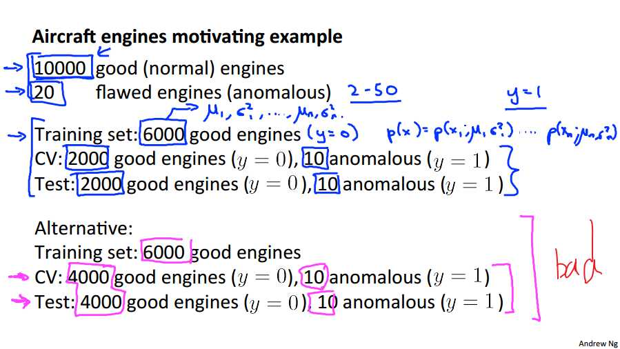
Let‘s say that, altogether, this is the data that we have. We have manufactured 10,000 examples of engines that, as far as we know we‘re perfectly normal, perfectly good aircraft engines. And again, it turns out to be okay even if a few flawed engine slips into the set of 10,000 is actually okay, but we kind of assumed that the vast majority of these 10,000 examples are, you know, good and normal non-anomalous engines. And let‘s say that, you know, historically, however long we‘ve been running on manufacturing plant, let‘s say that we end up getting features, getting 24 to 28 anomalous engines as well. And for a pretty typical application of anomaly detection, you know, the number non-anomalous examples, that is with y equals 1, we may have anywhere from, you know, 20 to 50. It would be a pretty typical range of examples, number of examples that we have with y equals 1. And usually we will have a much larger number of good examples. So, given this data set, a fairly typical way to split it into the training set, cross validation set and test set would be as follows. Let‘s take 10,000 good aircraft engines and put 6,000 of that into the unlabeled training set. So, I‘m calling this an unlabeled training set but all of these examples are really ones that correspond to y equals 0, as far as we know. And so, we will use this to fit p of x, right. So, we will use these 6000 engines to fit p of x, which is that p of x one parametrized by Mu 1, sigma squared 1, up to p of Xn parametrized by Mu N sigma squared n. And so it would be these 6,000 examples that we would use to estimate the parameters Mu 1, sigma squared 1, up to Mu N, sigma squared N. And so that‘s our training set of all, you know, good, or the vast majority of good examples. Next we will take our good aircraft engines and put some number of them in a cross validation set plus some number of them in the test sets. So 6,000 plus 2,000 plus 2,000, that‘s how we split up our 10,000 good aircraft engines. And then we also have 20 flawed aircraft engines, and we‘ll take that and maybe split it up, you know, put ten of them in the cross validation set and put ten of them in the test sets. And in the next slide we will talk about how to actually use this to evaluate the anomaly detection algorithm. So what I have just described here is a you know probably the recommend a good way of splitting the labeled and unlabeled example. The good and the flawed aircraft engines. Where we use like a 60, 20, 20% split for the good engines and we take the flawed engines, and we put them just in the cross validation set, and just in the test set, then we‘ll see in the next slide why that‘s the case. Just as an aside, if you look at how people apply anomaly detection algorithms, sometimes you see other peoples‘ split the data differently as well. So, another alternative, this is really not a recommended alternative, but some people want to take off your 10,000 good engines, maybe put 6000 of them in your training set and then put the same 4000 in the cross validation set and the test set. And so, you know, we like to think of the cross validation set and the test set as being completely different data sets to each other. But you know, in anomaly detection, you know, for sometimes you see people, sort of, use the same set of good engines in the cross validation sets, and the test sets, and sometimes you see people use exactly the same sets of anomalous engines in the cross validation set and the test set. And so, all of these are considered, you know, less good practices and definitely less recommended. Certainly using the same data in the cross validation set and the test set, that is not considered a good machine learning practice. But, sometimes you see people do this too.

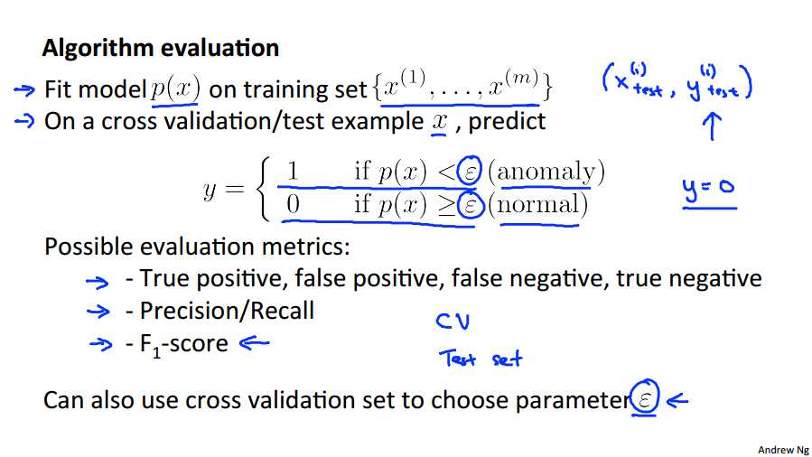
So, given the training cross validation and test sets, here‘s how you evaluate or here is how you develop and evaluate an algorithm. First, we take the training sets and we fit the model p of x. So, we fit, you know, all these Gaussians to my m unlabeled examples of aircraft engines, and these, I am calling them unlabeled examples, but these are really examples that we‘re assuming our goods are the normal aircraft engines. Then imagine that your anomaly detection algorithm is actually making prediction. So, on the cross validation of the test set, given that, say, test example X, think of the algorithm as predicting that y is equal to 1, p of x is less than epsilon, we must be taking zero, if p of x is greater than or equal to epsilon. So, given x, it‘s trying to predict, what is the label, given y equals 1 corresponding to an anomaly or is it y equals 0 corresponding to a normal example? So given the training, cross validation, and test sets. How do you develop an algorithm? And more specifically, how do you evaluate an anomaly detection algorithm? Well, to this whole, the first step is to take the unlabeled training set, and to fit the model p of x lead training data. So you take this, you know on I‘m coming, unlabeled training set, but really, these are examples that we are assuming, vast majority of which are normal aircraft engines, not because they‘re not anomalies and it will fit the model p of x. It will fit all those parameters for all the Gaussians on this data. Next on the cross validation of the test set, we‘re going to think of the anomaly detention algorithm as trying to predict the value of y. So in each of like say test examples. We have these X-I tests, Y-I test, where y is going to be equal to 1 or 0 depending on whether this was an anomalous example. So given input x in my test set, my anomaly detection algorithm think of it as predicting the y as 1 if p of x is less than epsilon. So predicting that it is an anomaly, it is probably is very low. And we think of the algorithm is predicting that y is equal to 0. If p of x is greater then or equals epsilon. So predicting those normal example if the p of x is reasonably large. And so we can now think of the anomaly detection algorithm as making predictions for what are the values of these y labels in the test sets or on the cross validation set. And this puts us somewhat more similar to the supervised learning setting, right? Where we have label test set and our algorithm is making predictions on these labels and so we can evaluate it you know by seeing how often it gets these labels right. Of course these labels are will be very skewed because y equals zero, that is normal examples, usually be much more common than y equals 1 than anomalous examples. But, you know, this is much closer to the source of evaluation metrics we can use in supervised learning. So what‘s a good evaluation metric to use. Well, because the data is very skewed, because y equals 0 is much more common, classification accuracy would not be a good the evaluation metrics. So, we talked about this in the earlier video. So, if you have a very skewed data set, then predicting y equals 0 all the time, will have very high classification accuracy. Instead, we should use evaluation metrics, like computing the fraction of true positives, false positives, false negatives, true negatives or compute the position of the v curve of this algorithm or do things like compute the f1 score, right, which is a single real number way of summarizing the position and the recall numbers. And so these would be ways to evaluate an anomaly detection algorithm on your cross validation set or on your test set. Finally, earlier in the anomaly detection algorithm, we also had this parameter epsilon, right? So, epsilon is this threshold that we would use to decide when to flag something as an anomaly. And so, if you have a cross validation set, another way to and to choose this parameter epsilon, would be to try a different, try many different values of epsilon, and then pick the value of epsilon that, let‘s say, maximizes f1 score, or that otherwise does well on your cross validation set. And more generally, the way to reduce the training, testing, and cross validation sets, is that when we are trying to make decisions, like what features to include, or trying to, you know, tune the parameter epsilon, we would then continually evaluate the algorithm on the cross validation sets and make all those decisions like what features did you use, you know, how to set epsilon, use that, evaluate the algorithm on the cross validation set, and then when we‘ve picked the set of features, when we‘ve found the value of epsilon that we‘re happy with, we can then take the final model and evaluate it, you know, do the final evaluation of the algorithm on the test sets. So, in this video, we talked about the process of how to evaluate an anomaly detection algorithm, and again, having being able to evaluate an algorithm, you know, with a single real number evaluation, with a number like an F1 score that often allows you to much more efficient use of your time when you are trying to develop an anomaly detection system. And we try to make these sorts of decisions. I have to chose epsilon, what features to include, and so on.

In this video, we started to use a bit of labeled data in order to evaluate the anomaly detection algorithm and this takes us a little bit closer to a supervised learning setting. In the next video, I‘m going to say a bit more about that. And in particular we‘ll talk about when should you be using an anomaly detection algorithm and when should we be thinking about using supervised learning instead, and what are the differences between these two formalisms.

summary

To evaluate our learning algorithm, we take some labeled data, categorized into anomalous and non-anomalous examples ( y = 0 if normal, y = 1 if anomalous).
Among that data, take a large proportion of good , non-anomalous data for the training set on which to train p(x).
Then, take a smaller proportion of mixed anomalous and non-anomalous examples (you will usually have many more non-anomalous examples) for your cross-validation and test sets.
For example, we may have a set where 0.2% of the data is anomalous. We take 60% of those examples, all of which are good (y=0) for the training set. We then take 20% of the examples for the cross-validation set (with 0.1% of the anomalous examples) and another 20% from the test set (with another 0.1% of the anomalous).
In other words, we split the data 60/20/20 training/CV/test and then split the anomalous examples 50/50 between the CV and test sets.
Algorithm evaluation:
Fit model p(x) on training set \\[\\lbrace x^{(1)},\\dots,x^{(m)} \\rbrace\\]
On a cross validation/test example x, predict:

• If \\(p(x) < ?\\) ( anomaly ), then \\(y = 1\\)
• If \\(p(x) ≥ ?\\) ( normal ), then \\(y = 0\\)

Possible evaluation metrics (see "Machine Learning System Design" section):

• True positive, false positive, false negative, true negative.
• Precision/recall
• \\(F_1\\) score

Note that we use the cross-validation set to choose parameter \\(?\\)

02_anomaly-detection-vs-supervised-learning

In the last video we talked about the process of evaluating an anomaly detection algorithm. And there we started to use some label data with examples that we knew were either anomalous or not anomalous with Y equals one, or Y equals 0. And so, the question then arises of, and if we have the label data, that we have some examples and know the anomalies, and some of them will not be anomalies. Why don‘t we just use a supervisor on half of them? So why don‘t we just use logistic regression, or a neuro network to try to learn directly from our labeled data to predict whether Y equals one or Y equals 0. In this video, I‘ll try to share with you some of the thinking and some guidelines for when you should probably use an anomaly detection algorithm, and whether it might be more fruitful instead of using a supervisor in the algorithm.

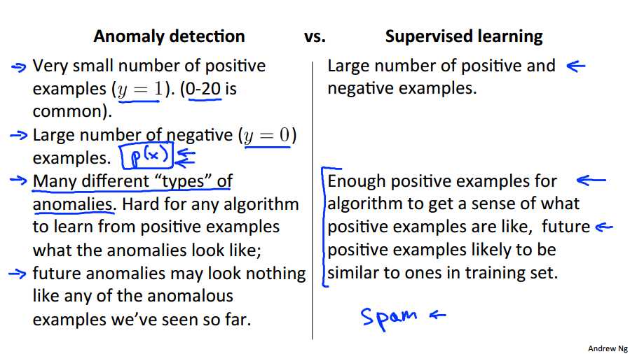
This slide shows what are the settings under which you should maybe use anomaly detection versus when supervised learning might be more fruitful. If you have a problem with a very small number of positive examples, and remember the examples of y equals one are the anomaly examples. Then you might consider using an anomaly detection algorithm instead. So, having 0 to 20, it may be up to 50 positive examples, might be pretty typical. And usually we have such a small positive, set of positive examples, we‘re going to save the positive examples just for the cross validation set in the test set. And in contrast, in a typical normal anomaly detection setting, we will often have a relatively large number of negative examples of the normal examples of normal aircraft engines. And we can then use this very large number of negative examples With which to fit the model p(x). And so there‘s this idea that in many anomaly detection applications, you have very few positive examples and lots of negative examples. And when we‘re doing the process of estimating p(x), affecting all those Gaussian parameters, we need only negative examples to do that. So if you have a lot negative data, we can still fit p(x) pretty well. In contrast, for supervised learning, more typically we would have a reasonably large number of both positive and negative examples. And so this is one way to look at your problem and decide if you should use an anomaly detection algorithm or a supervised. Here‘s another way that people often think about anomaly detection. So for anomaly detection applications, often there are very different types of anomalies. So think about so many different ways for go wrong. There are so many things that could go wrong that could the aircraft engine. And so if that‘s the case, and if you have a pretty small set of positive examples, then it can be hard for an algorithm, difficult for an algorithm to learn from your small set of positive examples what the anomalies look like. And in particular, you know future anomalies may look nothing like the ones you‘ve seen so far. So maybe in your set of positive examples, maybe you‘ve seen 5 or 10 or 20 different ways that an aircraft engine could go wrong. But maybe tomorrow, you need to detect a totally new set, a totally new type of anomaly. A totally new way for an aircraft engine to be broken, that you‘ve just never seen before. And if that‘s the case, it might be more promising to just model the negative examples with this sort of calcium model p of x rather than try to hard to model the positive examples. Because tomorrow‘s anomaly may be nothing like the ones you‘ve seen so far. In contrast, in some other problems, you have enough positive examples for an algorithm to get a sense of what the positive examples are like. In particular, if you think that future positive examples are likely to be similar to ones in the training set; then in that setting, it might be more reasonable to have a supervisor in the algorithm that looks at all of the positive examples, looks at all of the negative examples, and uses that to try to distinguish between positives and negatives. Hopefully, this gives you a sense of if you have a specific problem, should you think about using an anomaly detection algorithm, or a supervised learning algorithm. And a key difference really is that in anomaly detection, often we have such a small number of positive examples that it is not possible for a learning algorithm to learn that much from the positive examples. And so what we do instead is take a large set of negative examples and have it just learn a lot, learn p(x) from just the negative examples. Of the normal aircraft engines and we‘ve reserved the small number of positive examples for evaluating our algorithms to use in the either the transvalidation set or the test set. And just as a side comment about this many different types of easier. In some earlier videos we talked about the email spam examples. In those examples, there are actually many different types of spam email, right? There‘s spam email that‘s trying to sell you things. Spam email trying to steal your passwords, this is called fishing emails and many different types of spam emails. But for the spam problem we usually have enough examples of spam email to see most of these different types of spam email because we have a large set of examples of spam. And that‘s why we usually think of spam as a supervised learning setting even though there are many different types of.

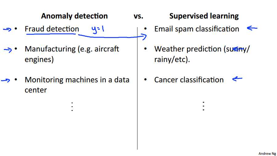
And so if we look at some applications of anomaly detection versus supervised learning we‘ll find fraud detection. If you have many different types of ways for people to try to commit fraud and a relatively small number of fraudulent users on your website, then I use an anomaly detection algorithm. I should say, if you have, if you‘re a very major online retailer and if you actually have had a lot of people commit fraud on your website, so you actually have a lot of examples of y=1, then sometimes fraud detection could actually shift over to the supervised learning algorithm. But, if you haven‘t seen that many examples of users doing strange things on your website, then more frequently fraud detection is actually treated as an anomaly detection algorithm rather than a supervised learning algorithm. Other examples, we‘ve talked about manufacturing already. Hopefully, you see more and more examples are not that many anomalies but if again for some manufacturing processes, if you manufacture in very large volumes and you see a lot of bad examples, maybe manufacturing can shift to the supervised learning column as well. But if you haven‘t seen that many bad examples of so to do the anomaly detection monitoring machines in a data center [INAUDIBLE] similar source of apply. Whereas, you must have classification, weather prediction, and classifying cancers. If you have equal numbers of positive and negative examples. Your positive and your negative examples, then we would tend to treat all of these as supervisor problems.

So hopefully, that gives you a sense of one of the properties of a learning problem that would cause you to treat it as an anomaly detection problem versus a supervisory problem. And for many other problems that are faced by various technology companies and so on, we actually are in the settings where we have very few or sometimes zero positive training examples. There‘s just so many different types of anomalies that we‘ve never seen them before. And for those sorts of problems, very often the algorithm that is used is an anomaly detection algorithm.

summary

When do we use anomaly detection and when do we use supervised learning?

Use anomaly detection when...

• We have a very small number of positive examples (y=1 ... 0-20 examples is common) and a large number of negative (y=0) examples.
• We have many different "types" of anomalies and it is hard for any algorithm to learn from positive examples what the anomalies look like; future anomalies may look nothing like any of the anomalous examples we‘ve seen so far.

Use supervised learning when...

• We have a large number of both positive and negative examples. In other words, the training set is more evenly divided into classes.
• We have enough positive examples for the algorithm to get a sense of what new positives examples look like. The future positive examples are likely similar to the ones in the training set.

03_choosing-what-features-to-use

By now you‘ve seen the anomaly detection algorithm and we‘ve also talked about how to evaluate an anomaly detection algorithm. It turns out, that when you‘re applying anomaly detection, one of the things that has a huge effect on how well it does, is what features you use, and what features you choose, to give the anomaly detection algorithm. So in this video, what I‘d like to do is say a few words, give some suggestions and guidelines for how to go about designing or selecting features give to an anomaly detection algorithm.

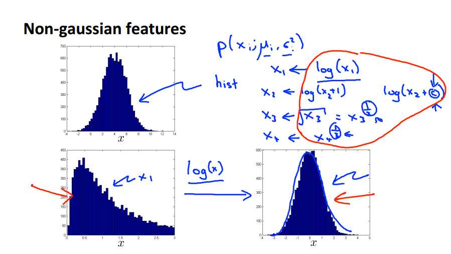
In our anomaly detection algorithm, one of the things we did was model the features using this sort of Gaussian distribution. With xi to mu i, sigma squared i, lets say. And so one thing that I often do would be to plot the data or the histogram of the data, to make sure that the data looks vaguely Gaussian before feeding it to my anomaly detection algorithm. And, it‘ll usually work okay, even if your data isn‘t Gaussian, but this is sort of a nice sanitary check to run. And by the way, in case your data looks non-Gaussian, the algorithms will often work just find. But, concretely if I plot the data like this, and if it looks like a histogram like this, and the way to plot a histogram is to use the HIST, or the HIST command in Octave, but it looks like this, this looks vaguely Gaussian, so if my features look like this, I would be pretty happy feeding into my algorithm. But if i were to plot a histogram of my data, and it were to look like this well, this doesn‘t look at all like a bell shaped curve, this is a very asymmetric distribution, it has a peak way off to one side. If this is what my data looks like, what I‘ll often do is play with different transformations of the data in order to make it look more Gaussian. And again the algorithm will usually work okay, even if you don‘t. But if you use these transformations to make your data more gaussian, it might work a bit better. So given the data set that looks like this, what I might do is take a log transformation of the data and if i do that and re-plot the histogram, what I end up with in this particular example, is a histogram that looks like this. And this looks much more Gaussian, right? This looks much more like the classic bell shaped curve, that we can fit with some mean and variance paramater sigma. So what I mean by taking a log transform, is really that if I have some feature x1 and then the histogram of x1 looks like this then I might take my feature x1 and replace it with log of x1 and this is my new x1 that I‘ll plot to the histogram over on the right, and this looks much more Guassian. Rather than just a log transform some other things you can do, might be, let‘s say I have a different feature x2, maybe I‘ll replace that will log x plus 1, or more generally with log x with x2 and some constant c and this constant could be something that I play with, to try to make it look as Gaussian as possible. Or for a different feature x3, maybe I‘ll replace it with x3, I might take the square root. The square root is just x3 to the power of one half, right? And this one half is another example of a parameter I can play with. So, I might have x4 and maybe I might instead replace that with x4 to the power of something else, maybe to the power of 1/3. And these, all of these, this one, this exponent parameter, or the C parameter, all of these are examples of parameters that you can play with in order to make your data look a little bit more Gaussian.

live demo

So, let me show you a live demo of how I actually go about playing with my data to make it look more Gaussian. So, I have already loaded in to octave here a set of features x I have a thousand examples loaded over there. So let‘s pull up the histogram of my data. Use the hist x command. So there‘s my histogram. By default, I think this uses 10 bins of histograms, but I want to see a more fine grid histogram. So we do hist to the x, 50, so, this plots it in 50 different bins.

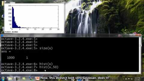
Okay, that looks better. Now, this doesn‘t look very Gaussian, does it? So, lets start playing around with the data. Lets try a hist of x to the 0.5. So we take the square root of the data, and plot that histogram.

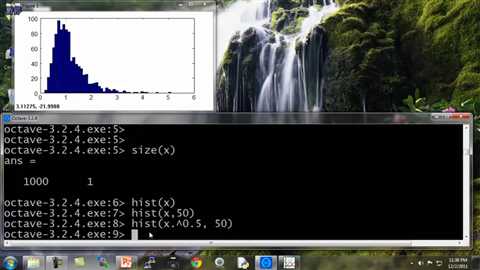
And, okay, it looks a little bit more Gaussian, but not quite there, so let‘s play at the 0.5 parameter. Let‘s see. Set this to 0.2.

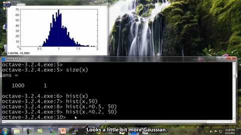
Looks a little bit more Gaussian. Let‘s reduce a little bit more 0.1. Yeah, that looks pretty good. I could actually just use 0.1.

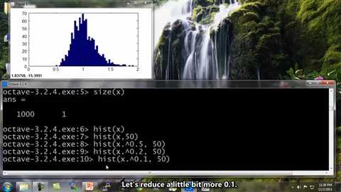
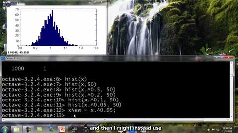
Well, let‘s reduce it to 0.05. And, you know? Okay, this looks pretty Gaussian, so I can define a new feature which is x mu equals x to the 0.05, and now my new feature x Mu looks more Gaussian than my previous one and then I might instead use this new feature to feed into my anomaly detection algorithm.

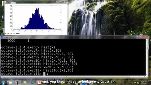
And of course, there is more than one way to do this. You could also have hist of log of x, that‘s another example of a transformation you can use. And, you know, that also look pretty Gaussian. So, I can also define x mu equals log of x. and that would be another pretty good choice of a feature to use.

So to summarize, if you plot a histogram with the data, and find that it looks pretty non-Gaussian, it‘s worth playing around a little bit with different transformations like these, to see if you can make your data look a little bit more Gaussian, before you feed it to your learning algorithm, although even if you don‘t, it might work okay. But I usually do take this step.

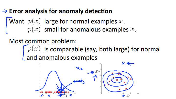
Now, the second thing I want to talk about is, how do you come up with features for an anomaly detection algorithm. And the way I often do so, is via an error analysis procedure. So what I mean by that, is that this is really similar to the error analysis procedure that we have for supervised learning, where we would train a complete algorithm, and run the algorithm on a cross validation set, and look at the examples it gets wrong, and see if we can come up with extra features to help the algorithm do better on the examples that it got wrong in the cross-validation set. So lets try to reason through an example of this process. In anomaly detection, we are hoping that p of x will be large for the normal examples and it will be small for the anomalous examples. And so a pretty common problem would be if p of x is comparable, maybe both are large for both the normal and the anomalous examples. Lets look at a specific example of that. Let‘s say that this is my unlabeled data. So, here I have just one feature, x1 and so I‘m gonna fit a Gaussian to this. And maybe my Gaussian that I fit to my data looks like that. And now let‘s say I have an anomalous example, and let‘s say that my anomalous example takes on an x value of 2.5. So I plot my anomalous example there. And you know, it‘s kind of buried in the middle of a bunch of normal examples, and so, just this anomalous example that I‘ve drawn in green, it gets a pretty high probability, where it‘s the height of the blue curve, and the algorithm fails to flag this as an anomalous example. Now, if this were maybe aircraft engine manufacturing or something, what I would do is, I would actually look at my training examples and look at what went wrong with that particular aircraft engine, and see, if looking at that example can inspire me to come up with a new feature x2, that helps to distinguish between this bad example, compared to the rest of my red examples, compared to all of my normal aircraft engines. And if I managed to do so, the hope would be then, that, if I can create a new feature, X2, so that when I re-plot my data, if I take all my normal examples of my training set, hopefully I find that all my training examples are these red crosses here. And hopefully, if I find that for my anomalous example, the feature x2 takes on the the unusual value. So for my green example here, this anomaly, right, my X1 value, is still 2.5. Then maybe my X2 value, hopefully it takes on a very large value like 3.5 over there, or a very small value. But now, if I model my data, I‘ll find that my anomaly detection algorithm gives high probability to data in the central regions, slightly lower probability to that, sightly lower probability to that. An example that‘s all the way out there, my algorithm will now give very low probability to. And so, the process of this is, really look at the mistakes that it is making. Look at the anomaly that the algorithm is failing to flag, and see if that inspires you to create some new feature. So find something unusual about that aircraft engine and use that to create a new feature, so that with this new feature it becomes easier to distinguish the anomalies from your good examples. And so that‘s the process of error analysis and using that to create new features for anomaly detection.

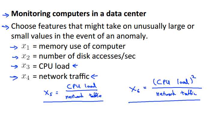
Finally, let me share with you my thinking on how I usually go about choosing features for anomaly detection. So, usually, the way I think about choosing features is I want to choose features that will take on either very, very large values, or very, very small values, for examples that I think might turn out to be anomalies. So let‘s use our example again of monitoring the computers in a data center. And so you have lots of machines, maybe thousands, or tens of thousands of machines in a data center. And we want to know if one of the machines, one of our computers is acting up, so doing something strange. So here are examples of features you may choose, maybe memory used, number of disc accesses, CPU load, network traffic. But now, lets say that I suspect one of the failure cases, let‘s say that in my data set I think that CPU load the network traffic tend to grow linearly with each other. Maybe I‘m running a bunch of web servers, and so, here if one of my servers is serving a lot of users, I have a very high CPU load, and have a very high network traffic. But let‘s say, I think, let‘s say I have a suspicion, that one of the failure cases is if one of my computers has a job that gets stuck in some infinite loop. So if I think one of the failure cases, is one of my machines, one of my web servers--server code-- gets stuck in some infinite loop, and so the CPU load grows, but the network traffic doesn‘t because it‘s just spinning it‘s wheels and doing a lot of CPU work, you know, stuck in some infinite loop. In that case, to detect that type of anomaly, I might create a new feature, X5, which might be CPU load divided by network traffic. And so here X5 will take on a unusually large value if one of the machines has a very large CPU load but not that much network traffic and so this will be a feature that will help your anomaly detection capture, a certain type of anomaly. And you can also get creative and come up with other features as well. Like maybe I have a feature x6 thats CPU load squared divided by network traffic. And this would be another variant of a feature like x5 to try to capture anomalies where one of your machines has a very high CPU load, that maybe doesn‘t have a commensurately large network traffic. And by creating features like these, you can start to capture anomalies that correspond to unusual combinations of values of the features.

So in this video we talked about how to and take a feature, and maybe transform it a little bit, so that it becomes a bit more Gaussian, before feeding into an anomaly detection algorithm. And also the error analysis in this process of creating features to try to capture different types of anomalies. And with these sorts of guidelines hopefully that will help you to choose good features, to give to your anomaly detection algorithm, to help it capture all sorts of anomalies.

summary

The features will greatly affect how well your anomaly detection algorithm works.
We can check that our features are gaussian by plotting a histogram of our data and checking for the bell-shaped curve.
Some transforms we can try on an example feature x that does not have the bell-shaped curve are:

• \\(log(x)\\)
• \\(log(x+1)\\)
• \\(log(x+c)\\) for some constant
• \\(\\sqrt{x}\\)
• \\(x^{1/3}\\)

We can play with each of these to try and achieve the gaussian shape in our data.
There is an error analysis procedure for anomaly detection that is very similar to the one in supervised learning.
Our goal is for \\(p(x)\\) to be large for normal examples and small for anomalous examples.
One common problem is when \\(p(x)\\) is similar for both types of examples. In this case, you need to examine the anomalous examples that are giving high probability in detail and try to figure out new features that will better distinguish the data.
In general, choose features that might take on unusually large or small values in the event of an anomaly.

03_multivariate-gaussian-distribution-optional

01_multivariate-gaussian-distribution

In this and the next video, I‘d like to tell you about one possible extension to the anomaly detection algorithm that we‘ve developed so far. This extension uses something called the multivariate Gaussian distribution, and it has some advantages, and some disadvantages, and it can sometimes catch some anomalies that the earlier algorithm didn‘t.

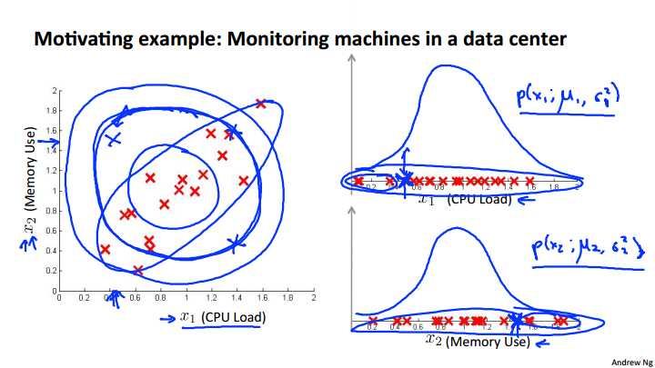
To motivate this, let‘s start with an example. Let‘s say that so our unlabeled data looks like what I have plotted here. And I‘m going to use the example of monitoring machines in the data center, monitoring computers in the data center. So my two features are x1 which is the CPU load and x2 which is maybe the memory use. So if I take my two features, x1 and x2, and I model them as Gaussians then here‘s a plot of my X1 features, here‘s a plot of my X2 features, and so if I fit a Gaussian to that, maybe I‘ll get a Gaussian like this, so here‘s P of X 1, which depends on the parameters mu 1, and sigma squared 1, and here‘s my memory used, and, you know, maybe I‘ll get a Gaussian that looks like this, and this is my P of X 2, which depends on mu 2 and sigma squared 2. And so this is how the anomaly detection algorithm models X1 and X2. Now let‘s say that in the test sets I have an example that looks like this. The location of that green cross, so the value of X 1 is about 0.4, and the value of X 2 is about 1.5. Now, if you look at the data, it looks like, yeah, most of the data data lies in this region, and so that green cross is pretty far away from any of the data I‘ve seen. It looks like that should be raised as an anomaly. So, in my data, in my, in the data of my good examples, it looks like, you know, the CPU load, and the memory use, they sort of grow linearly with each other. So if I have a machine using lots of CPU, you know memory use will also be high, whereas this example, this green example it looks like here, the CPU load is very low, but the memory use is very high, and I just have not seen that before in my training set. It looks like that should be an anomaly. But let‘s see what the anomaly detection algorithm will do. Well, for the CPU load, it puts it at around there 0.5 and this reasonably high probability is not that far from other examples we‘ve seen, maybe, whereas, for the memory use, this appointment, 0.5, whereas for the memory use, it‘s about 1.5, which is there. Again, you know, it‘s all to us, it‘s not terribly Gaussian, but the value here and the value here is not that different from many other examples we‘ve seen, and so P of X 1, will be pretty high, reasonably high. P of X 2 reasonably high. I mean, if you look at this plot right, this point here, it doesn‘t look that bad, and if you look at this plot, you know across here, doesn‘t look that bad. I mean, I have had examples with even greater memory used, or with even less CPU use, and so this example doesn‘t look that anomalous. And so, an anomaly detection algorithm will fail to flag this point as an anomaly. And it turns out what our anomaly detection algorithm is doing is that it is not realizing that this blue ellipse shows the high probability region, is that, one of the thing is that, examples here, a high probability, and the examples, the next circle of from a lower probably, and examples here are even lower probability, and somehow, here are things that are, green cross there, it‘s pretty high probability, and in particular, it tends to think that, you know, everything in this region, everything on the line that I‘m circling over, has, you know, about equal probability, and it doesn‘t realize that something out here actually has much lower probability than something over there.

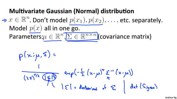
So, in order to fix this, we can, we‘re going to develop a modified version of the anomaly detection algorithm, using something called the multivariate Gaussian distribution also called the multivariate normal distribution. So here‘s what we‘re going to do. We have features x which are in Rn and instead of P of X 1, P of X 2, separately, we‘re going to model P of X, all in one go, so model P of X, you know, all at the same time. So the parameters of the multivariate Gaussian distribution are mu, which is a vector, and sigma, which is an n by n matrix, called a covariance matrix, and this is similar to the covariance matrix that we saw when we were working with the PCA, with the principal components analysis algorithm. For the second complete is, let me just write out the formula for the multivariate Gaussian distribution. So we say that probability of X, and this is parameterized by my parameters mu and sigma that the probability of x is equal to once again there‘s absolutely no need to memorize this formula. You know, you can look it up whenever you need to use it, but this is what the probability of X looks like. Transverse, 2nd inverse, X minus mu. And this thing here, the absolute value of sigma, this thing here when you write this symbol, this is called the determent of sigma and this is a mathematical function of a matrix and you really don‘t need to know what the determinant of a matrix is, but really all you need to know is that you can compute it in octave by using the octave command DET of sigma. Okay, and again, just be clear, alright? In this expression, these sigmas here, these are just n by n matrix. This is not a summation and you know, the sigma there is an n by n matrix. So that‘s the formula for P of X, but it‘s more interestingly, or more importantly, what does P of X actually looks like? Lets look at some examples of multivariate Gaussian distributions.

\\[p(x)=∏_{j=1}^{n}p(x_j;μ_j,σ^2_j)=∏_{j=1}^{n}\\frac{1}{\\sqrt{2π}σ_j}exp(-\\frac{(x_j-μ_j)^2}{2σ_j^2}), μ=\\frac{1}{m}\\sum_{i=1}^{m}x^{(i)} \\\\ p(x)=\\frac{1}{(2π)^{\\frac{n}{2}} |Σ|^{\\frac{1}{2}}}exp(-\\frac{1}{2}(x-μ)^TΣ^{-1}(x-μ)), Σ=\\frac{1}{m}(X-μ)^T(X-μ)\\]

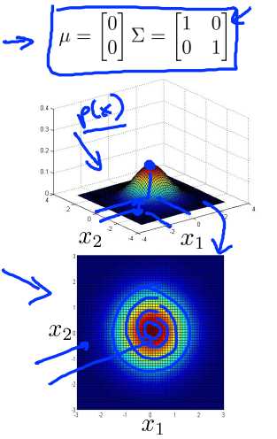
So let‘s take a two dimensional example, say if I have N equals 2, I have two features, X1 and X2. Lets say I set MU to be equal to 0 and sigma to be equal to this matrix here. With 1s on the diagonals and 0s on the off-diagonals, this matrix is sometimes also called the identity matrix. In that case, p of x will look like this, and what I‘m showing in this figure is, you know, for a specific value of X1 and for a specific value of X2, the height of this surface the value of p of x. And so with this setting the parameters p of x is highest when X1 and X2 equal zero 0, so that‘s the peak of this Gaussian distribution, and the probability falls off with this sort of two dimensional Gaussian or this bell shaped two dimensional bell-shaped surface. Down below is the same thing but plotted using a contour plot instead, or using different colors, and so this heavy intense red in the middle, corresponds to the highest values, and then the values decrease with the yellow being slightly lower values the cyan being lower values and this deep blue being the lowest values so this is really the same figure but plotted viewed from the top instead, using colors instead. And so, with this distribution, you see that it faces most of the probability near 0,0 and then as you go out from 0,0 the probability of X1 and X2 goes down.

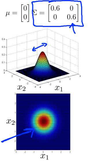
Now lets try varying some of the parameters and see what happens. So let‘s take sigma and change it so let‘s say sigma shrinks a little bit. Sigma is a covariance matrix and so it measures the variance or the variability of the features X1 X2. So if the shrink sigma then what you get is what you get is that the width of this bump diminishes and the height also increases a bit, because the area under the surface is equal to 1. So the integral of the volume under the surface is equal to 1, because probability distribution must integrate to one. But, if you shrink the variance, it‘s kinda like shrinking sigma squared, you end up with a narrower distribution, and one that‘s a little bit taller. And so you see here also the concentric ellipsis has shrunk a little bit.

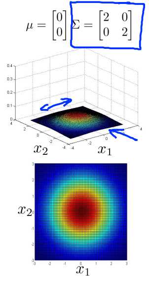
Whereas in contrast if you were to increase sigma to 2 2 on the diagonals, so it is now two times the identity then you end up with a much wider and much flatter Gaussian. And so the width of this is much wider. This is hard to see but this is still a bell shaped bump, it‘s just flattened down a lot, it has become much wider and so the variance or the variability of X1 and X2 just becomes wider. Here are a few more examples.

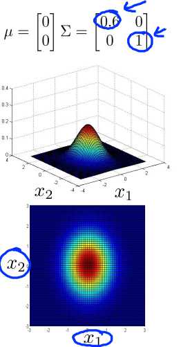
Now lets try varying one of the elements of sigma at the time. Let‘s say I send sigma to 0.6 there, and 1 over there. What this does, is this reduces the variance of the first feature, X 1, while keeping the variance of the second feature X 2, the same. And so with this setting of parameters, you can model things like that. X 1 has smaller variance, and X 2 has larger variance.

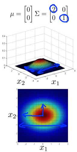
Whereas if I do this, if I set this matrix to 2, 1 then you can also model examples where you know here we‘ll say X1 can have take on a large range of values whereas X2 takes on a relatively narrower range of values. And that‘s reflected in this figure as well, you know where, the distribution falls off more slowly as X 1 moves away from 0, and falls off very rapidly as X 2 moves away from 0.

And similarly if we were to modify this element of the matrix instead, then similar to the previous slide, except that here where you know playing around here saying that X2 can take on a very small range of values and so here if this is 0.6, we notice now X2 tends to take on a much smaller range of values than the original example, whereas if we were to set sigma to be equal to 2 then that‘s like saying X2 you know, has a much larger range of values.

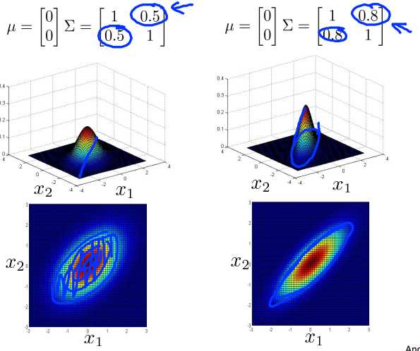
Now, one of the cool things about the multivariate Gaussian distribution is that you can also use it to model correlations between the data. That is we can use it to model the fact that X1 and X2 tend to be highly correlated with each other for example. So specifically if you start to change the off diagonal entries of this covariance matrix you can get a different type of Gaussian distribution. And so as I increase the off-diagonal entries from .5 to .8, what I get is this distribution that is more and more thinly peaked along this sort of x equals y line. And so here the contour says that x and y tend to grow together and the things that are with large probability are if either X1 is large and Y2 is large or X1 is small and Y2 is small. Or somewhere in between. And as this entry, 0.8 gets large, you get a Gaussian distribution, that‘s sort of where all the probability lies on this sort of narrow region, where x is approximately equal to y. This is a very tall, thin distribution you know line mostly along this line central region where x is close to y. So this is if we set these entries to be positive entries.

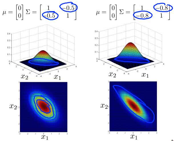
In contrast if we set these to negative values, as I decreases it to -.5 down to -.8, then what we get is a model where we put most of the probability in this sort of negative X one in the next 2 correlation region, and so, most of the probability now lies in this region, where X 1 is about equal to -X 2, rather than X 1 equals X 2. And so this captures a sort of negative correlation between x1 and x2. And so this is a hopefully this gives you a sense of the different distributions that the multivariate Gaussian distribution can capture.

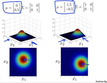
So follow up in varying, the covariance matrix sigma, the other thing you can do is also, vary the mean parameter mu, and so operationally, we have mu equal 0 0, and so the distribution was centered around X 1 equals 0, X2 equals 0, so the peak of the distribution is here, whereas, if we vary the values of mu, then that varies the peak of the distribution and so, if mu equals 0, 0.5, the peak is at, you know, X1 equals zero, and X2 equals 0.5, and so the peak or the center of this distribution has shifted, and if mu was 1.5 minus 0.5 then OK, and similarly the peak of the distribution has now shifted to a different location, corresponding to where, you know, X1 is 1.5 and X2 is -0.5, and so varying the mu parameter, just shifts around the center of this whole distribution.

So, hopefully, looking at all these different pictures gives you a sense of the sort of probability distributions that the Multivariate Gaussian Distribution allows you to capture. And the key advantage of it is it allows you to capture, when you‘d expect two different features to be positively correlated, or maybe negatively correlated.

In the next video, we‘ll take this multivariate Gaussian distribution and apply it to anomaly detection.

summary

The multivariate gaussian distribution is an extension of anomaly detection and may (or may not) catch more anomalies.
Instead of modeling \\(p(x_1),p(x_2),\\dots\\) separately, we will model p(x) all in one go. Our parameters will be: \\(\\mu \\in \\mathbb{R}^n\\) and \\(\\Sigma \\in \\mathbb{R}^{n \\times n}\\)
\\[p(x;\\mu,\\Sigma) = \\dfrac{1}{(2\\pi)^{n\\over 2} |\\Sigma|^{1\\over 2}} exp(-{1\\over 2}(x-\\mu)^T\\Sigma^{-1}(x-\\mu))\\]
The important effect is that we can model oblong gaussian contours, allowing us to better fit data that might not fit into the normal circular contours.

Varying Σ changes the shape, width, and orientation of the contours. Changing μ will move the center of the distribution.

Check also:

• The Multivariate Gaussian Distribution http://cs229.stanford.edu/section/gaussians.pdf Chuong B. Do, October 10, 2008.

02_anomaly-detection-using-the-multivariate-gaussian-distribution

In the last video we talked about the Multivariate Gaussian Distribution and saw some examples of the sorts of distributions you can model, as you vary the parameters, mu and sigma. In this video, let‘s take those ideas, and apply them to develop a different anomaly detection algorithm.

To recap the multivariate Gaussian distribution and the multivariate normal distribution has two parameters, mu and sigma. Where mu this an n dimensional vector and sigma, the covariance matrix, is an n by n matrix. And here‘s the formula for the probability of X, as parameterized by mu and sigma, and as you vary mu and sigma, you can get a range of different distributions, like, you know, these are three examples of the ones that we saw in the previous video. So let‘s talk about the parameter fitting or the parameter estimation problem. The question, as usual, is if I have a set of examples X1 through XM and here each of these examples is an n dimensional vector and I think my examples come from a multivariate Gaussian distribution. How do I try to estimate my parameters mu and sigma? Well the standard formulas for estimating them is you set mu to be just the average of your training examples. And you set sigma to be equal to this. And this is actually just like the sigma that we had written out, when we were using the PCA or the Principal Components Analysis algorithm. So you just plug in these two formulas and this would give you your estimated parameter mu and your estimated parameter sigma. So given the data set here is how you estimate mu and sigma.

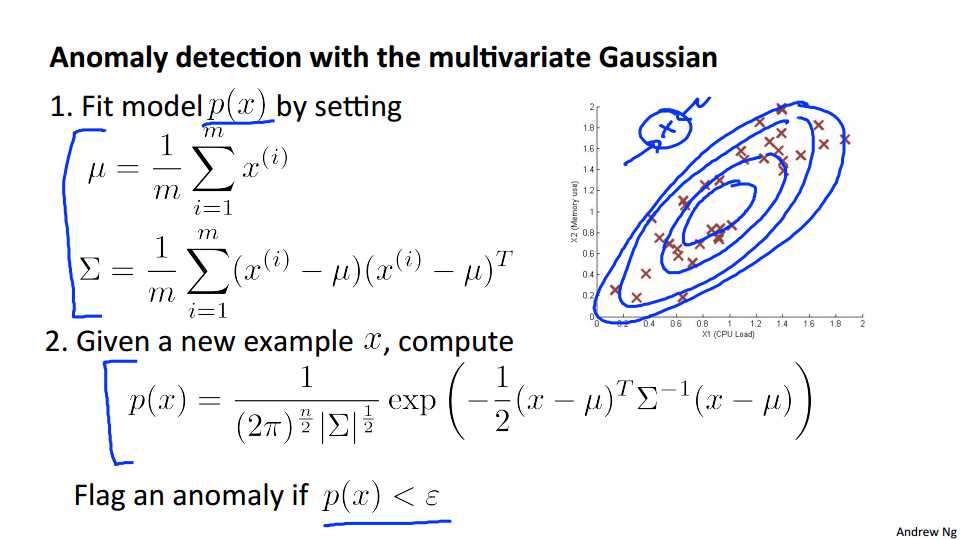
Let‘s take this method and just plug it into an anomaly detection algorithm. So how do we put all of this together to develop an anomaly detection algorithm? Here ‘s what we do. First we take our training set, and we fit the model, we fit P of X, by, you know, setting mu and sigma as described on the previous slide. Next when you are given a new example X. So if you are given a test example, lets take an earlier example to have a new example out here. And that is my test example. Given the new example X, what we are going to do is compute P of X, using this formula for the multivariate Gaussian distribution. And then, if P of X is very small, then we flagged it as an anomaly, whereas, if P of X is greater than that parameter epsilon, then we don‘t flag it as an anomaly. So it turns out, if we were to fit a multivariate Gaussian distribution to this data set, so just the red crosses, not the green example, you end up with a Gaussian distribution that places lots of probability in the central region, slightly less probability here, slightly less probability here, slightly less probability here, and very low probability at the point that is way out here. And so, if you apply the multivariate Gaussian distribution to this example, it will actually correctly flag that example. as an anomaly.

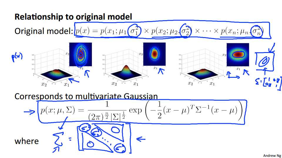
Finally it‘s worth saying a few words about what is the relationship between the multivariate Gaussian distribution model, and the original model, where we were modeling P of X as a product of this P of X1, P of X2, up to P of Xn. It turns out that you can prove mathematically, I‘m not going to do the proof here, but you can prove mathematically that this relationship, between the multivariate Gaussian model and this original one. And in particular, it turns out that the original model corresponds to multivariate Gaussians, where the contours of the Gaussian are always axis aligned. So all three of these are examples of Gaussian distributions that you can fit using the original model. It turns out that that corresponds to multivariate Gaussian, where, you know, the ellipsis here, the contours of this distribution--it turns out that this model actually corresponds to a special case of a multivariate Gaussian distribution. And in particular, this special case is defined by constraining the distribution of p of x, the multivariate a Gaussian distribution of p of x, so that the contours of the probability density function, of the probability distribution function, are axis aligned. And so you can get a p of x with a multivariate Gaussian that looks like this, or like this, or like this. And you notice, that in all 3 of these examples, these ellipses, or these ovals that I‘m drawing, have their axes aligned with the X1 X2 axes. And what we do not have, is a set of contours that are at an angle, right? And this corresponded to examples where sigma is equal to 1 1, 0.8, 0.8. Let‘s say, with non-0 elements on the off diagonals. So, it turns out that it‘s possible to show mathematically that this model actually is the same as a multivariate Gaussian distribution but with a constraint. And the constraint is that the covariance matrix sigma must have 0‘s on the off diagonal elements. In particular, the covariance matrix sigma, this thing here, it would be sigma squared 1, sigma squared 2, down to sigma squared n, and then everything on the off diagonal entries, all of these elements above and below the diagonal of the matrix, all of those are going to be zero. And in fact if you take these values of sigma, sigma squared 1, sigma squared 2, down to sigma squared n, and plug them into here, and you know, plug them into this covariance matrix, then the two models are actually identical. That is, this new model, using a multivariate Gaussian distribution, corresponds exactly to the old model, if the covariance matrix sigma, has only 0 elements off the diagonals, and in pictures that corresponds to having Gaussian distributions, where the contours of this distribution function are axis aligned. So you aren‘t allowed to model the correlations between the diffrent features. So in that sense the original model is actually a special case of this multivariate Gaussian model.

So when would you use each of these two models? So when would you the original model and when would you use the multivariate Gaussian model?

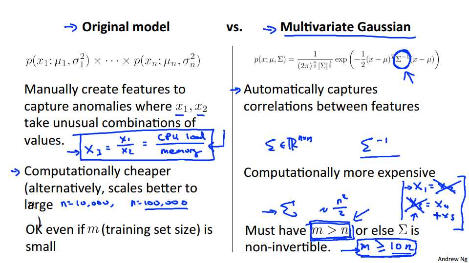
The original model is probably used somewhat more often, and whereas the multivariate Gaussian distribution is used somewhat less but it has the advantage of being able to capture correlations between features. So suppose you want to capture anomalies where you have different features say where features x1, x2 take on unusual combinations of values so in the earlier example, we had that example where the anomaly was with the CPU load and the memory use taking on unusual combinations of values, if you want to use the original model to capture that, then what you need to do is create an extra feature, such as X3 equals X1/X2, you know equals maybe the CPU load divided by the memory used, or something, and you need to create extra features if there‘s unusual combinations of values where X1 and X2 take on an unusual combination of values even though X1 by itself and X2 by itself looks like it‘s taking a perfectly normal value. But if you‘re willing to spend the time to manually create an extra feature like this, then the original model will work fine. Whereas in contrast, the multivariate Gaussian model can automatically capture correlations between different features. But the original model has some other more significant advantages, too, and one huge advantage of the original model is that it is computationally cheaper, and another view on this is that is scales better to very large values of n and very large numbers of features, and so even if n were ten thousand, or even if n were equal to a hundred thousand, the original model will usually work just fine. Whereas in contrast for the multivariate Gaussian model notice here, for example, that we need to compute the inverse of the matrix sigma where sigma is an n by n matrix and so computing sigma if sigma is a hundred thousand by a hundred thousand matrix that is going to be very computationally expensive. And so the multivariate Gaussian model scales less well to large values of N. And finally for the original model, it turns out to work out ok even if you have a relatively small training set this is the small unlabeled examples that we use to model p of x of course, and this works fine, even if M is, you know, maybe 50, 100, works fine. Whereas for the multivariate Gaussian, it is sort of a mathematical property of the algorithm that you must have m greater than n, so that the number of examples is greater than the number of features you have. And there‘s a mathematical property of the way we estimate the parameters that if this is not true, so if m is less than or equal to n, then this matrix isn‘t even invertible, that is this matrix is singular, and so you can‘t even use the multivariate Gaussian model unless you make some changes to it. But a typical rule of thumb that I use is, I will use the multivariate Gaussian model only if m is much greater than n, so this is sort of the narrow mathematical requirement, but in practice, I would use the multivariate Gaussian model, only if m were quite a bit bigger than n. So if m were greater than or equal to 10 times n, let‘s say, might be a reasonable rule of thumb, and if it doesn‘t satisfy this, then the multivariate Gaussian model has a lot of parameters, right, so this covariance matrix sigma is an n by n matrix, so it has, you know, roughly n squared parameters, because it‘s a symmetric matrix, it‘s actually closer to n squared over 2 parameters, but this is a lot of parameters, so you need make sure you have a fairly large value for m, make sure you have enough data to fit all these parameters. And m greater than or equal to 10 n would be a reasonable rule of thumb to make sure that you can estimate this covariance matrix sigma reasonably well. So in practice the original model shown on the left that is used more often. And if you suspect that you need to capture correlations between features what people will often do is just manually design extra features like these to capture specific unusual combinations of values. But in problems where you have a very large training set or m is very large and n is not too large, then the multivariate Gaussian model is well worth considering and may work better as well, and can save you from having to spend your time to manually create extra features in case the anomalies turn out to be captured by unusual combinations of values of the features. Finally I just want to briefly mention one somewhat technical property, but if you‘re fitting multivariate Gaussian model, and if you find that the covariance matrix sigma is singular, or you find it‘s non-invertible, they‘re usually 2 cases for this. One is if it‘s failing to satisfy this m greater than n condition, and the second case is if you have redundant features. So by redundant features, I mean, if you have 2 features that are the same. Somehow you accidentally made two copies of the feature, so your x1 is just equal to x2. Or if you have redundant features like maybe your features X3 is equal to feature X4, plus feature X5. Okay, so if you have highly redundant features like these, you know, where if X3 is equal to X4 plus X5, well X3 doesn‘t contain any extra information, right? You just take these 2 other features, and add them together. And if you have this sort of redundant features, duplicated features, or this sort of features, than sigma may be non-invertible. And so there‘s a debugging set-- this should very rarely happen, so you probably won‘t run into this, it is very unlikely that you have to worry about this-- but in case you implement a multivariate Gaussian model you find that sigma is non-invertible. What I would do is first make sure that M is quite a bit bigger than N, and if it is then, the second thing I do, is just check for redundant features. And so if there are 2 features that are equal, just get rid of one of them, or if you have redundant if these , X3 equals X4 plus X5, just get rid of the redundant feature, and then it should work fine again. As an aside for those of you who are experts in linear algebra, by redundant features, what I mean is the formal term is features that are linearly dependent. But in practice what that really means is one of these problems tripping up the algorithm if you just make you features non-redundant., that should solve the problem of sigma being non-invertable. But once again the odds of your running into this at all are pretty low so chances are, you can just apply the multivariate Gaussian model, without having to worry about sigma being non-invertible, so long as m is greater than or equal to n. So that‘s it for anomaly detection, with the multivariate Gaussian distribution. And if you apply this method you would be able to have an anomaly detection algorithm that automatically captures positive and negative correlations between your different features and flags an anomaly if it sees is unusual combination of the values of the features.

summary

When doing anomaly detection with multivariate gaussian distribution, we compute \\(μ\\) and \\(Σ\\) normally. We then compute \\(p(x)\\) using the new formula in the previous section and flag an anomaly if \\(p(x) < ?\\).
The original model for p(x) corresponds to a multivariate Gaussian where the contours of \\(p(x;\\mu,\\Sigma)\\) are axis-aligned.
The multivariate Gaussian model can automatically capture correlations between different features of \\(x\\).
However, the original model maintains some advantages: it is computationally cheaper (no matrix to invert, which is costly for large number of features) and it performs well even with small training set size (in multivariate Gaussian model, it should be greater than the number of features for \\(Σ\\) to be invertible