手把手教你搭建神经网络（CT扫描3D图像的分类）

Posted 2021-05-20 羽峰码字

tags:

篇首语：本文由小常识网(cha138.com)小编为大家整理，主要介绍了手把手教你搭建神经网络（CT扫描3D图像的分类）相关的知识，希望对你有一定的参考价值。

大家好，我是羽峰，今天要和大家分享的是一个基于tensorflow的CT扫描3D图像的分类。文章会把整个代码进行分割讲解，完整看完，相信你一定会有所收获。

欢迎关注“羽峰码字”

1. 项目简介

此示例将显示构建3D卷积神经网络（CNN）以预测计算机断层扫描（CT）扫描中病毒性肺炎的存在所需的步骤。 2D CNN通常用于处理RGB图像（3通道）。 3D CNN只是3D等效项：它以3D体积或2D帧序列（例如CT扫描中的切片）为输入，因此3D CNN是学习体积数据表示的强大模型。

2. API准备

import os
import zipfile
import numpy as np
import tensorflow as tf

from tensorflow import keras
from tensorflow.keras import layers

3. 数据集准备

3.1 下载数据

下载MosMedData：具有COVID-19相关发现的胸部CT扫描

在此示例中，我们使用了MosMedData: Chest CT Scans with COVID-19 Related Findings。该数据集包含具有COVID-19相关发现以及没有发现的肺部CT扫描。

我们将使用CT扫描的相关放射学发现作为标记，以建立分类器来预测病毒性肺炎的存在。因此，该任务是二进制分类问题。

# Download url of normal CT scans.
url = "https://github.com/hasibzunair/3D-image-classification-tutorial/releases/download/v0.2/CT-0.zip"
filename = os.path.join(os.getcwd(), "CT-0.zip")
keras.utils.get_file(filename, url)

# Download url of abnormal CT scans.
url = "https://github.com/hasibzunair/3D-image-classification-tutorial/releases/download/v0.2/CT-23.zip"
filename = os.path.join(os.getcwd(), "CT-23.zip")
keras.utils.get_file(filename, url)

# Make a directory to store the data.
os.makedirs("MosMedData")

# Unzip data in the newly created directory.
with zipfile.ZipFile("CT-0.zip", "r") as z_fp:
    z_fp.extractall("./MosMedData/")

with zipfile.ZipFile("CT-23.zip", "r") as z_fp:
    z_fp.extractall("./MosMedData/")

3.2 数据预处理

这些文件以Nifti格式提供，扩展名为.nii。要读取扫描结果，我们使用nibabel软件包。您可以通过pip install nibabel安装软件包。 CT扫描以Hounsfield单位（HU）存储原始体素强度。在此数据集中，它们的范围从-1024到2000以上。高于400的骨骼具有不同的放射强度，因此将其用作更高的界限。通常将-1000到400之间的阈值用于归一化CT扫描。

要处理数据，我们执行以下操作：

我们首先将体积旋转90度，因此方向是固定的
我们将HU值缩放为介于0和1之间。
我们调整宽度，高度和深度的大小。

在这里，我们定义了几个辅助函数来处理数据。在构建训练和验证数据集时将使用这些功能。

import nibabel as nib

from scipy import ndimage


def read_nifti_file(filepath):
    """Read and load volume"""
    # Read file
    scan = nib.load(filepath)
    # Get raw data
    scan = scan.get_fdata()
    return scan


def normalize(volume):
    """Normalize the volume"""
    min = -1000
    max = 400
    volume[volume < min] = min
    volume[volume > max] = max
    volume = (volume - min) / (max - min)
    volume = volume.astype("float32")
    return volume


def resize_volume(img):
    """Resize across z-axis"""
    # Set the desired depth
    desired_depth = 64
    desired_width = 128
    desired_height = 128
    # Get current depth
    current_depth = img.shape[-1]
    current_width = img.shape[0]
    current_height = img.shape[1]
    # Compute depth factor
    depth = current_depth / desired_depth
    width = current_width / desired_width
    height = current_height / desired_height
    depth_factor = 1 / depth
    width_factor = 1 / width
    height_factor = 1 / height
    # Rotate
    img = ndimage.rotate(img, 90, reshape=False)
    # Resize across z-axis
    img = ndimage.zoom(img, (width_factor, height_factor, depth_factor), order=1)
    return img


def process_scan(path):
    """Read and resize volume"""
    # Read scan
    volume = read_nifti_file(path)
    # Normalize
    volume = normalize(volume)
    # Resize width, height and depth
    volume = resize_volume(volume)
    return volume

让我们从类目录中读取CT扫描的路径。

# Folder "CT-0" consist of CT scans having normal lung tissue,
# no CT-signs of viral pneumonia.
normal_scan_paths = [
    os.path.join(os.getcwd(), "MosMedData/CT-0", x)
    for x in os.listdir("MosMedData/CT-0")
]
# Folder "CT-23" consist of CT scans having several ground-glass opacifications,
# involvement of lung parenchyma.
abnormal_scan_paths = [
    os.path.join(os.getcwd(), "MosMedData/CT-23", x)
    for x in os.listdir("MosMedData/CT-23")
]

print("CT scans with normal lung tissue: " + str(len(normal_scan_paths)))
print("CT scans with abnormal lung tissue: " + str(len(abnormal_scan_paths)))

3.3 建立训练和验证数据集

从类目录中读取扫描并分配标签。对扫描进行下采样以具有128x128x64的形状。将原始HU值重新缩放为0到1的范围。最后，将数据集拆分为训练和验证子集。

# Read and process the scans.
# Each scan is resized across height, width, and depth and rescaled.
abnormal_scans = np.array([process_scan(path) for path in abnormal_scan_paths])
normal_scans = np.array([process_scan(path) for path in normal_scan_paths])

# For the CT scans having presence of viral pneumonia
# assign 1, for the normal ones assign 0.
abnormal_labels = np.array([1 for _ in range(len(abnormal_scans))])
normal_labels = np.array([0 for _ in range(len(normal_scans))])

# Split data in the ratio 70-30 for training and validation.
x_train = np.concatenate((abnormal_scans[:70], normal_scans[:70]), axis=0)
y_train = np.concatenate((abnormal_labels[:70], normal_labels[:70]), axis=0)
x_val = np.concatenate((abnormal_scans[70:], normal_scans[70:]), axis=0)
y_val = np.concatenate((abnormal_labels[70:], normal_labels[70:]), axis=0)
print(
    "Number of samples in train and validation are %d and %d."
    % (x_train.shape[0], x_val.shape[0])
)

3.4 数据增强

在训练过程中，CT扫描也可以通过以任意角度旋转来增强。由于数据存储在形状（样本，高度，宽度，深度）的3级张量中，因此我们在轴4上添加了尺寸为1的尺寸，以便能够对数据执行3D卷积。因此，新形状为（样本，高度，宽度，深度，1）。还有有各种各样的预处理和扩充技术请读者们查阅相关资料，此示例显示了一些简单的入门和增强技术。

import random

from scipy import ndimage


@tf.function
def rotate(volume):
    """Rotate the volume by a few degrees"""

    def scipy_rotate(volume):
        # define some rotation angles
        angles = [-20, -10, -5, 5, 10, 20]
        # pick angles at random
        angle = random.choice(angles)
        # rotate volume
        volume = ndimage.rotate(volume, angle, reshape=False)
        volume[volume < 0] = 0
        volume[volume > 1] = 1
        return volume

    augmented_volume = tf.numpy_function(scipy_rotate, [volume], tf.float32)
    return augmented_volume


def train_preprocessing(volume, label):
    """Process training data by rotating and adding a channel."""
    # Rotate volume
    volume = rotate(volume)
    volume = tf.expand_dims(volume, axis=3)
    return volume, label


def validation_preprocessing(volume, label):
    """Process validation data by only adding a channel."""
    volume = tf.expand_dims(volume, axis=3)
    return volume, label

在定义训练和验证数据加载器时，训练数据会通过和增强功能传递，该功能会随机旋转不同角度的体积。请注意，训练和验证数据均已重新缩放为0到1之间的值。

# Define data loaders.
train_loader = tf.data.Dataset.from_tensor_slices((x_train, y_train))
validation_loader = tf.data.Dataset.from_tensor_slices((x_val, y_val))

batch_size = 2
# Augment the on the fly during training.
train_dataset = (
    train_loader.shuffle(len(x_train))
    .map(train_preprocessing)
    .batch(batch_size)
    .prefetch(2)
)
# Only rescale.
validation_dataset = (
    validation_loader.shuffle(len(x_val))
    .map(validation_preprocessing)
    .batch(batch_size)
    .prefetch(2)
)

可视化CT增强图像

import matplotlib.pyplot as plt

data = train_dataset.take(1)
images, labels = list(data)[0]
images = images.numpy()
image = images[0]
print("Dimension of the CT scan is:", image.shape)
plt.imshow(np.squeeze(image[:, :, 30]), cmap="gray")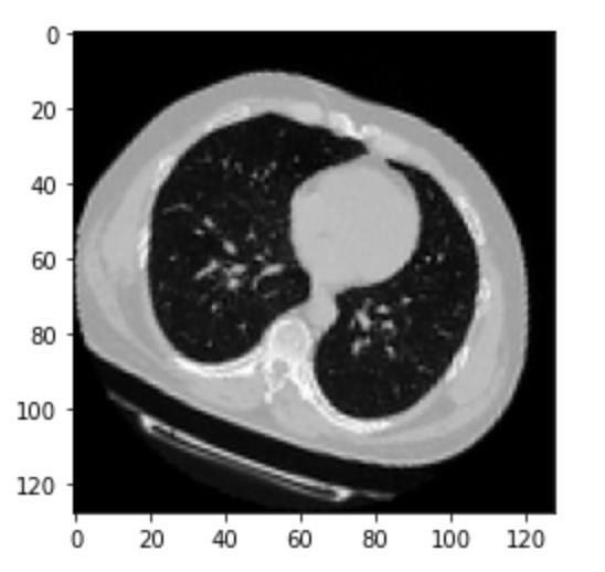

由于CT扫描有很多切片，用序列形式进行排列显示

def plot_slices(num_rows, num_columns, width, height, data):
    """Plot a montage of 20 CT slices"""
    data = np.rot90(np.array(data))
    data = np.transpose(data)
    data = np.reshape(data, (num_rows, num_columns, width, height))
    rows_data, columns_data = data.shape[0], data.shape[1]
    heights = [slc[0].shape[0] for slc in data]
    widths = [slc.shape[1] for slc in data[0]]
    fig_width = 12.0
    fig_height = fig_width * sum(heights) / sum(widths)
    f, axarr = plt.subplots(
        rows_data,
        columns_data,
        figsize=(fig_width, fig_height),
        gridspec_kw={"height_ratios": heights},
    )
    for i in range(rows_data):
        for j in range(columns_data):
            axarr[i, j].imshow(data[i][j], cmap="gray")
            axarr[i, j].axis("off")
    plt.subplots_adjust(wspace=0, hspace=0, left=0, right=1, bottom=0, top=1)
    plt.show()


# Visualize montage of slices.
# 4 rows and 10 columns for 100 slices of the CT scan.
plot_slices(4, 10, 128, 128, image[:, :, :40])

4 模型构建

4.1 定义3D卷积神经网络

为了使模型更易于理解，我们将其构造为块。本示例中使用的3D CNN的体系结构是基于本文的。

def get_model(width=128, height=128, depth=64):
    """Build a 3D convolutional neural network model."""

    inputs = keras.Input((width, height, depth, 1))

    x = layers.Conv3D(filters=64, kernel_size=3, activation="relu")(inputs)
    x = layers.MaxPool3D(pool_size=2)(x)
    x = layers.BatchNormalization()(x)

    x = layers.Conv3D(filters=64, kernel_size=3, activation="relu")(x)
    x = layers.MaxPool3D(pool_size=2)(x)
    x = layers.BatchNormalization()(x)

    x = layers.Conv3D(filters=128, kernel_size=3, activation="relu")(x)
    x = layers.MaxPool3D(pool_size=2)(x)
    x = layers.BatchNormalization()(x)

    x = layers.Conv3D(filters=256, kernel_size=3, activation="relu")(x)
    x = layers.MaxPool3D(pool_size=2)(x)
    x = layers.BatchNormalization()(x)

    x = layers.GlobalAveragePooling3D()(x)
    x = layers.Dense(units=512, activation="relu")(x)
    x = layers.Dropout(0.3)(x)

    outputs = layers.Dense(units=1, activation="sigmoid")(x)

    # Define the model.
    model = keras.Model(inputs, outputs, name="3dcnn")
    return model


# Build model.
model = get_model(width=128, height=128, depth=64)
model.summary()

4.2 训练模型

# Compile model.
initial_learning_rate = 0.0001
lr_schedule = keras.optimizers.schedules.ExponentialDecay(
    initial_learning_rate, decay_steps=100000, decay_rate=0.96, staircase=True
)
model.compile(
    loss="binary_crossentropy",
    optimizer=keras.optimizers.Adam(learning_rate=lr_schedule),
    metrics=["acc"],
)

# Define callbacks.
checkpoint_cb = keras.callbacks.ModelCheckpoint(
    "3d_image_classification.h5", save_best_only=True
)
early_stopping_cb = keras.callbacks.EarlyStopping(monitor="val_acc", patience=15)

# Train the model, doing validation at the end of each epoch
epochs = 100
model.fit(
    train_dataset,
    validation_data=validation_dataset,
    epochs=epochs,
    shuffle=True,
    verbose=2,
    callbacks=[checkpoint_cb, early_stopping_cb],
)

4.3 验证模型

在此绘制了训练和验证集的模型准确性和损失。由于验证集是类平衡的，因此准确性提供了模型性能的公正表示。

fig, ax = plt.subplots(1, 2, figsize=(20, 3))
ax = ax.ravel()

for i, metric in enumerate(["acc", "loss"]):
    ax[i].plot(model.history.history[metric])
    ax[i].plot(model.history.history["val_" + metric])
    ax[i].set_title("Model {}".format(metric))
    ax[i].set_xlabel("epochs")
    ax[i].set_ylabel(metric)
    ax[i].legend(["train", "val"])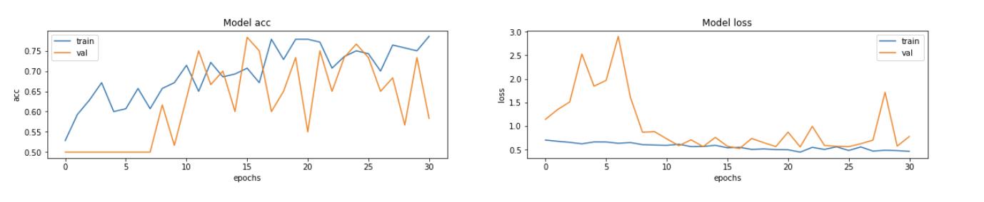

5. 使用模型进行预测

# Load best weights.
model.load_weights("3d_image_classification.h5")
prediction = model.predict(np.expand_dims(x_val[0], axis=0))[0]
scores = [1 - prediction[0], prediction[0]]

class_names = ["normal", "abnormal"]
for score, name in zip(scores, class_names):
    print(
        "This model is %.2f percent confident that CT scan is %s"
        % ((100 * score), name)
    )

References

- A survey on Deep Learning Advances on Different 3D DataRepresentations(https://arxiv.org/pdf/1808.01462.pdf)
- VoxNet: A 3D Convolutional Neural Network for Real-Time Object Recognition(https://www.ri.cmu.edu/pub_files/2015/9/voxnet_maturana_scherer_iros15.pdf)
- FusionNet: 3D Object Classification Using MultipleData Representations(http://3ddl.cs.princeton.edu/2016/papers/Hegde_Zadeh.pdf)
- Uniformizing Techniques to Process CT scans with 3D CNNs for Tuberculosis Prediction(https://arxiv.org/abs/2007.13224)
至此,今天的分享结束了,希望通过以上分享,你能学习到语义分割的基本流程,基本过程,与图像分割类似,但更具象化。强烈建议新手能按照上述步骤一步步实践下来,必有收获。
今天代码翻译于:https://keras.io/examples/vision/3D_image_classification/,新入门的小伙伴可以好好看看这个网站,很基础,很适合新手。
当然,这里不得不重点推荐一下这三个网站:
https://tensorflow.google.cn/tutorials/keras/classification
https://keras.io/examples
https://keras.io/zh/
其中keras中文网址中能找到各种API定义,都是中文通俗易懂,如果想看英文直接到https://keras.io/,就可以,这里也有很多案例,也是很基础明白。入门时可以看看。
我是羽峰,还在成长道路上摸爬滚打的小白,希望能够结识一起成长的你,公众号“羽峰码字”,欢迎来撩。
以上是关于手把手教你搭建神经网络(CT扫描3D图像的分类)的主要内容,如果未能解决你的问题,请参考以下文章
手把手教你搭建神经网络(使用Vision Transformer进行图像分类)