Pytorch+PyG实现MLP

Posted 2023-04-01 海洋.之心

文章目录

• 前言
• 一、导入相关库
• 二、加载Cora数据集
• 三、定义MLP网络
• 四、定义模型
• 五、模型训练
• 六、模型验证
• 七、结果
• 完整代码

---

前言

大家好，我是阿光。

本专栏整理了《图神经网络代码实战》，内包含了不同图神经网络的相关代码实现（PyG以及自实现），理论与实践相结合，如GCN、GAT、GraphSAGE等经典图网络，每一个代码实例都附带有完整的代码。

正在更新中~ ✨

🚨 我的项目环境：

• 平台：Windows10
• 语言环境：python3.7
• 编译器：PyCharm
• PyTorch版本：1.11.0
• PyG版本：2.1.0

💥 项目专栏：【图神经网络代码实战目录】

---

本文我们将使用Pytorch + Pytorch Geometric来简易实现一个MLP（感知机网络），让新手可以理解如何PyG来搭建一个简易的图网络实例demo。

一、导入相关库

本项目我们需要结合两个库，一个是Pytorch，因为还需要按照torch的网络搭建模型进行书写，第二个是PyG，因为在torch中并没有关于图网络层的定义，所以需要torch_geometric这个库来定义一些图层。

import torch
import torch.nn.functional as F
import torch.nn as nn
import torch_geometric.nn as pyg_nn
from torch_geometric.datasets import Planetoid

二、加载Cora数据集

本文使用的数据集是比较经典的Cora数据集，它是一个根据科学论文之间相互引用关系而构建的Graph数据集合，论文分为7类，共2708篇。

• Genetic_Algorithms
• Neural_Networks
• Probabilistic_Methods
• Reinforcement_Learning
• Rule_Learning
• Theory

这个数据集是一个用于图节点分类的任务，数据集中只有一张图，这张图中含有2708个节点，10556条边，每个节点的特征维度为1433。

# 1.加载Cora数据集
dataset = Planetoid(root='./data/Cora', name='Cora')

三、定义MLP网络

这里我们就不重点介绍MLP网络了，相信大家能够掌握基本原理，本文我们使用的是PyG定义网络层，在PyG中已经定义好了MLP这个层，该层采用的就是感知机机制。

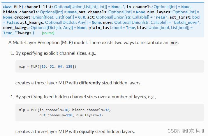
对于MLP的常用参数：

• channel_list：样本输入层、中间层、输出层维度的列表
• in_channels：每个样本的输入维度，就是每个节点的特征维度
• hidden_channels：单层神经网络中间的隐层大小
• out_channels：经过MLP后映射成的新的维度，就是经过MLP后每个节点的维度长度
• num_layers：感知机层数
• dropout：每个隐藏层的丢弃率，如果存在多层可以使用列表传入
• act：激活函数，默认为relu
• bias：训练一个偏置b

对于本文实现的 pyg_nn.MLP([num_node_features, 32, 64, 128]) 的含义就是定义一个三层的感知机网络，按照 PyTorch 实现等价于如下代码：

lin_1 = nn.Linear(num_node_features, 32)
lin_2 = nn.Linear(32, 64)
lin_3 = nn.Linear(64, 128)

对于 PyG 中实现起来较为简单，以列表方式传入所以隐层大小即可，第一个维度代表样本的输入特征维度，最后一个维度代表输出的维度大小，中间维度代表隐层的大小，所以 len(channel_list) - 1 代表 MLP 的层数，这种方式是以传入 channel_list 方式定义模型，还可以按照正常参数方式进行传递定义，代码如下：

pyg_nn.MLP(in_channels=16,
		   hidden_channels=32,
		   out_channels=128,
		   num_layers=3)

网络定义代码如下：

# 2.定义MLP网络
class MLP(nn.Module):
    def __init__(self, num_node_features, num_classes):
        super(MLP, self).__init__()
        self.lin_1 = pyg_nn.MLP([num_node_features, 32, 64, 128])
        self.lin_2 = pyg_nn.MLP([128, 64, 32, num_classes])
        
    def forward(self, data):
        x, edge_index = data.x, data.edge_index
        
        x = self.lin_1(x, edge_index)
        x = F.relu(x)
        x = F.dropout(x, training=self.training)
        x = self.lin_2(x, edge_index)
        
        return F.log_softmax(x, dim=1)

上面网络我们定义了两个MLP层，第一层的参数的输入维度就是初始每个节点的特征维度，输出维度是128。

第二个层的输入维度为128，输出维度为分类个数，因为我们需要对每个节点进行分类，最终加上softmax操作。

四、定义模型

下面就是定义了一些模型需要的参数，像学习率、迭代次数这些超参数，然后是模型的定义以及优化器及损失函数的定义，和pytorch定义网络是一样的。

device = torch.device('cuda' if torch.cuda.is_available() else 'cpu') # 设备
epochs = 10 # 学习轮数
lr = 0.003 # 学习率
num_node_features = dataset.num_node_features # 每个节点的特征数
num_classes = dataset.num_classes # 每个节点的类别数
data = dataset[0].to(device) # Cora的一张图

# 3.定义模型
model = MLP(num_node_features, num_classes).to(device)
optimizer = torch.optim.Adam(model.parameters(), lr=lr) # 优化器
loss_function = nn.NLLLoss() # 损失函数

五、模型训练

模型训练部分也是和pytorch定义网络一样，因为都是需要经过前向传播、反向传播这些过程，对于损失、精度这些指标可以自己添加。

# 训练模式
model.train()

for epoch in range(epochs):
    optimizer.zero_grad()
    pred = model(data)
    
    loss = loss_function(pred[data.train_mask], data.y[data.train_mask]) # 损失
    correct_count_train = pred.argmax(axis=1)[data.train_mask].eq(data.y[data.train_mask]).sum().item() # epoch正确分类数目
    acc_train = correct_count_train / data.train_mask.sum().item() # epoch训练精度
    
    loss.backward()
    optimizer.step()
    
    if epoch % 20 == 0:
        print("【EPOCH: 】%s" % str(epoch + 1))
        print('训练损失为：:.4f'.format(loss.item()), '训练精度为：:.4f'.format(acc_train))

print('【Finished Training！】')

六、模型验证

下面就是模型验证阶段，在训练时我们是只使用了训练集，测试的时候我们使用的是测试集，注意这和传统网络测试不太一样，在图像分类一些经典任务中，我们是把数据集分成了两份，分别是训练集、测试集，但是在Cora这个数据集中并没有这样，它区分训练集还是测试集使用的是掩码机制，就是定义了一个和节点长度相同纬度的数组，该数组的每个位置为True或者False，标记着是否使用该节点的数据进行训练。

# 模型验证
model.eval()
pred = model(data)

# 训练集（使用了掩码）
correct_count_train = pred.argmax(axis=1)[data.train_mask].eq(data.y[data.train_mask]).sum().item()
acc_train = correct_count_train / data.train_mask.sum().item()
loss_train = loss_function(pred[data.train_mask], data.y[data.train_mask]).item()

# 测试集
correct_count_test = pred.argmax(axis=1)[data.test_mask].eq(data.y[data.test_mask]).sum().item()
acc_test = correct_count_test / data.test_mask.sum().item()
loss_test = loss_function(pred[data.test_mask], data.y[data.test_mask]).item()

print('Train Accuracy: :.4f'.format(acc_train), 'Train Loss: :.4f'.format(loss_train))
print('Test  Accuracy: :.4f'.format(acc_test), 'Test  Loss: :.4f'.format(loss_test))

七、结果

【EPOCH: 】1
训练损失为：1.9856 训练精度为：0.1786
【EPOCH: 】21
训练损失为：1.5419 训练精度为：0.4643
【EPOCH: 】41
训练损失为：1.1653 训练精度为：0.6500
【EPOCH: 】61
训练损失为：0.8062 训练精度为：0.8071
【EPOCH: 】81
训练损失为：0.5322 训练精度为：0.9286
【EPOCH: 】101
训练损失为：0.3487 训练精度为：0.9714
【EPOCH: 】121
训练损失为：0.2132 训练精度为：0.9571
【EPOCH: 】141
训练损失为：0.1043 训练精度为：0.9929
【EPOCH: 】161
训练损失为：0.0601 训练精度为：1.0000
【EPOCH: 】181
训练损失为：0.0420 训练精度为：1.0000
【Finished Training！】

>>>Train Accuracy: 1.0000 Train Loss: 0.0092
>>>Test  Accuracy: 0.1800 Test  Loss: 1.9587

	训练集	测试集
Accuracy	1.0000	0.1800
Loss	0.0092	1.9587

完整代码

import torch
import torch.nn.functional as F
import torch.nn as nn
import torch_geometric.nn as pyg_nn
from torch_geometric.datasets import Planetoid

# 1.加载Cora数据集
dataset = Planetoid(root='./data/Cora', name='Cora')

# 2.定义MLP网络
class MLP(nn.Module):
    def __init__(self, num_node_features, num_classes):
        super(MLP, self).__init__()
        self.lin_1 = pyg_nn.MLP([num_node_features, 32, 64, 128])
        self.lin_2 = pyg_nn.MLP([128, 64, 32, num_classes])
        
    def forward(self, data):
        x, edge_index = data.x, data.edge_index
        
        x = self.lin_1(x, edge_index)
        x = F.relu(x)
        x = F.dropout(x, training=self.training)
        x = self.lin_2(x, edge_index)
        
        return F.log_softmax(x, dim=1)

device = torch.device('cuda' if torch.cuda.is_available() else 'cpu') # 设备
epochs = 200 # 学习轮数
lr = 0.0003 # 学习率
num_node_features = dataset.num_node_features # 每个节点的特征数
num_classes = dataset.num_classes # 每个节点的类别数
data = dataset[0].to(device) # Cora的一张图

# 3.定义模型
model = MLP(num_node_features, num_classes).to(device)
optimizer = torch.optim.Adam(model.parameters(), lr=lr) # 优化器
loss_function = nn.NLLLoss() # 损失函数

# 训练模式
model.train()

for epoch in range(epochs):
    optimizer.zero_grad()
    pred = model(data)
    
    loss = loss_function(pred[data.train_mask], data.y[data.train_mask]) # 损失
    correct_count_train = pred.argmax(axis=1)[data.train_mask].eq(data.y[data.train_mask]).sum().item() # epoch正确分类数目
    acc_train = correct_count_train / data.train_mask.sum().item() # epoch训练精度
    
    loss.backward()
    optimizer.step()
    
    if epoch % 20 == 0:
        print("【EPOCH: 】%s" % str(epoch + 1))
        print('训练损失为：:.4f'.format(loss.item()), '训练精度为：:.4f'.format(acc_train))

print('【Finished Training！】')

# 模型验证
model.eval()
pred = model(data)

# 训练集（使用了掩码）
correct_count_train = pred.argmax(axis=1)[data.train_mask].eq(data.y[data.train_mask]).sum().item()
acc_train = correct_count_train / data.train_mask.sum().item()
loss_train = loss_function(pred[data.train_mask], data.y[data.train_mask]).item()

# 测试集
correct_count_test = pred.argmax(axis=1)[data.test_mask].eq(data.y[data.test_mask]).sum().item()
acc_test = correct_count_test / data.test_mask.sum().item()
loss_test = loss_function(pred[data.test_mask], data.y[data.test_mask]).item()

print('Train Accuracy: :.4f'.format(acc_train), 'Train Loss: :.4f'.format(loss_train))
print('Test  Accuracy: :.4f'.format(acc_test), 'Test  Loss: :.4f'.format(loss_test))

从头开始实现 MLP 和在 PyTorch 中实现有啥区别？

【中文标题】从头开始实现 MLP 和在 PyTorch 中实现有啥区别？

【英文标题】：What is the difference between MLP implementation from scratch and in PyTorch?从头开始实现 MLP 和在 PyTorch 中实现有什么区别？

【发布时间】：2019-06-12 07:33:57

【问题描述】：

跟进How to update the learning rate in a two layered multi-layered perceptron?的问题

鉴于 XOR 问题：

X = xor_input = np.array([[0,0], [0,1], [1,0], [1,1]])
Y = xor_output = np.array([[0,1,1,0]]).T

还有一个简单的

两层多层感知器 (MLP) 与 它们和 之间的 sigmoid 激活 均方误差 (MSE) 作为损失函数/优化标准

如果我们这样从头开始训练模型：

from itertools import chain
import matplotlib.pyplot as plt
import numpy as np
np.random.seed(0)

def sigmoid(x): # Returns values that sums to one.
    return 1 / (1 + np.exp(-x))

def sigmoid_derivative(sx):
    # See https://math.stackexchange.com/a/1225116
    return sx * (1 - sx)

# Cost functions.
def mse(predicted, truth):
    return 0.5 * np.mean(np.square(predicted - truth))

def mse_derivative(predicted, truth):
    return predicted - truth

X = xor_input = np.array([[0,0], [0,1], [1,0], [1,1]])
Y = xor_output = np.array([[0,1,1,0]]).T

# Define the shape of the weight vector.
num_data, input_dim = X.shape
# Lets set the dimensions for the intermediate layer.
hidden_dim = 5
# Initialize weights between the input layers and the hidden layer.
W1 = np.random.random((input_dim, hidden_dim))

# Define the shape of the output vector. 
output_dim = len(Y.T)
# Initialize weights between the hidden layers and the output layer.
W2 = np.random.random((hidden_dim, output_dim))

# Initialize weigh
num_epochs = 5000
learning_rate = 0.3

losses = []

for epoch_n in range(num_epochs):
    layer0 = X
    # Forward propagation.

    # Inside the perceptron, Step 2. 
    layer1 = sigmoid(np.dot(layer0, W1))
    layer2 = sigmoid(np.dot(layer1, W2))

    # Back propagation (Y -> layer2)

    # How much did we miss in the predictions?
    cost_error = mse(layer2, Y)
    cost_delta = mse_derivative(layer2, Y)

    #print(layer2_error)
    # In what direction is the target value?
    # Were we really close? If so, don't change too much.
    layer2_error = np.dot(cost_delta, cost_error)
    layer2_delta = cost_delta *  sigmoid_derivative(layer2)

    # Back propagation (layer2 -> layer1)
    # How much did each layer1 value contribute to the layer2 error (according to the weights)?
    layer1_error = np.dot(layer2_delta, W2.T)
    layer1_delta = layer1_error * sigmoid_derivative(layer1)

    # update weights
    W2 += - learning_rate * np.dot(layer1.T, layer2_delta)
    W1 += - learning_rate * np.dot(layer0.T, layer1_delta)
    #print(np.dot(layer0.T, layer1_delta))
    #print(epoch_n, list((layer2)))

    # Log the loss value as we proceed through the epochs.
    losses.append(layer2_error.mean())
    #print(cost_delta)


# Visualize the losses
plt.plot(losses)
plt.show()

从 epoch 0 开始，我们的损失急剧下降，然后迅速饱和：

但是如果我们用pytorch训练一个类似的模型，训练曲线在饱和之前损失会逐渐下降：

从头开始的 MLP 和 PyTorch 代码有什么区别？

为什么会在不同点收敛？

除了权重初始化、代码中的np.random.rand() 和默认的手电筒初始化之外，我似乎看不出模型有什么不同。

PyTorch 代码：

from tqdm import tqdm
import numpy as np

import torch
from torch import nn
from torch import tensor
from torch import optim

import matplotlib.pyplot as plt

torch.manual_seed(0)
device = 'gpu' if torch.cuda.is_available() else 'cpu'

# XOR gate inputs and outputs.
X = xor_input = tensor([[0,0], [0,1], [1,0], [1,1]]).float().to(device)
Y = xor_output = tensor([[0],[1],[1],[0]]).float().to(device)


# Use tensor.shape to get the shape of the matrix/tensor.
num_data, input_dim = X.shape
print('Inputs Dim:', input_dim) # i.e. n=2 

num_data, output_dim = Y.shape
print('Output Dim:', output_dim) 
print('No. of Data:', num_data) # i.e. n=4

# Step 1: Initialization. 

# Initialize the model.
# Set the hidden dimension size.
hidden_dim = 5
# Use Sequential to define a simple feed-forward network.
model = nn.Sequential(
            # Use nn.Linear to get our simple perceptron.
            nn.Linear(input_dim, hidden_dim),
            # Use nn.Sigmoid to get our sigmoid non-linearity.
            nn.Sigmoid(),
            # Second layer neurons.
            nn.Linear(hidden_dim, output_dim),
            nn.Sigmoid()
        )
model

# Initialize the optimizer
learning_rate = 0.3
optimizer = optim.SGD(model.parameters(), lr=learning_rate)

# Initialize the loss function.
criterion = nn.MSELoss()

# Initialize the stopping criteria
# For simplicity, just stop training after certain no. of epochs.
num_epochs = 5000 

losses = [] # Keeps track of the loses.

# Step 2-4 of training routine.

for _e in tqdm(range(num_epochs)):
    # Reset the gradient after every epoch. 
    optimizer.zero_grad() 
    # Step 2: Foward Propagation
    predictions = model(X)

    # Step 3: Back Propagation 
    # Calculate the cost between the predictions and the truth.
    loss = criterion(predictions, Y)
    # Remember to back propagate the loss you've computed above.
    loss.backward()

    # Step 4: Optimizer take a step and update the weights.
    optimizer.step()

    # Log the loss value as we proceed through the epochs.
    losses.append(loss.data.item())


plt.plot(losses)

【问题讨论】：

如果您能告诉我们在手动编码示例中潜水有多锐利，这可能会有所帮助。 2个时代？ 20？对我来说，图表的明显解释是学习率在某种程度上非常不同。 （另外，作为单独的说明：MSE 损失在这里可能不是适当的错误函数，并且您将希望在实践中对 $[0, 1]$ 中的输出使用负对数损失/交叉熵损失，但是对于这么简单的问题，它并不重要，当然它与问题并不特别相关。）

你的从头开始的代码抛出---> 60 layer1_error = np.dot(layer2_delta, W2.T) ..... ValueError: shapes (4,50) and (1,5) not aligned: 50 (dim 1) != 1 (dim 0)

@alvas 在训练结束时，理想情况下你的损失应该在0.0 左右，对吧？这是否意味着 PyTorch 代码有问题？ @coldspeed 我能够从从头开始的代码中重现 OP 的结果。当你运行它时，layer2_delta 似乎以某种方式以(4, 50) 结束（对我来说layer2_delta.shape 是(4,1)）。

好的，花了一点时间，但我想出了如何让您的手动代码产生与 Pytorch 代码相同的结果。有 4 个显着差异需要说明。这都是一些小的调整，所以看起来你的手工代码的核心是好的（除了必须加倍学习率的东西：这可能是某个地方的数学错误）。

【参考方案1】：

手卷代码和 PyTorch 代码的区别列表

事实证明，您的手动代码和 PyTorch 代码所做的事情之间存在很多差异。以下是我发现的内容，大致按对输出的影响从大到小的顺序列出：

您的代码和 PyTorch 代码使用两个不同的函数来报告丢失。 您的代码和 PyTorch 代码设置的初始权重非常不同。您在问题中提到了这一点，但事实证明它对结果产生了相当大的影响。 默认情况下，torch.nn.Linear 层会为模型添加额外的一堆“偏差”权重。因此，Pytorch 模型的第一层有效地具有3x5 权重，而第二层具有6x1 权重。手卷代码中的层分别具有2x5 和5x1 权重。 偏差似乎有助于模型更快地学习和适应。如果关闭偏差，Pytorch 模型需要大约两倍的训练 epoch 才能达到0 损失附近。 奇怪的是，看起来 Pytorch 模型使用的学习率实际上是您指定的一半。或者，也可能是 2 的杂散因子在您的手卷数学/代码中某处被发现。

如何从手卷和 Pytorch 代码中得到相同的结果

通过仔细考虑以上 4 个因素，可以实现手卷代码和 Pytorch 代码的完全对等。通过正确的调整和设置，两个 sn-ps 将产生相同的结果：

最重要的调整 - 使损失报告功能匹配

关键的区别在于你最终使用两个完全不同的函数来测量两个代码 sn-ps 中的损失：

在手卷代码中，您将损失测量为layer2_error.mean()。如果你解压变量，你可以看到 layer2_error.mean() 是一个有点古怪和毫无意义的值：

layer2_error.mean()
== np.dot(cost_delta, cost_error).mean()
== np.dot(mse_derivative(layer2, Y), mse(layer2, Y)).mean()
== np.sum(.5 * (layer2 - Y) * ((layer2 - Y)**2).mean()).mean()

另一方面，在 PyTorch 代码中，损失是根据 mse 的传统定义来衡量的，即等同于 np.mean((layer2 - Y)**2)。您可以通过如下方式修改 PyTorch 循环来向自己证明这一点：

def mse(x, y):
    return np.mean((x - y)**2)

torch_losses = [] # Keeps track of the loses.
torch_losses_manual = [] # for comparison

# Step 2-4 of training routine.

for _e in tqdm(range(num_epochs)):
    # Reset the gradient after every epoch. 
    optimizer.zero_grad() 
    # Step 2: Foward Propagation
    predictions = model(X)

    # Step 3: Back Propagation 
    # Calculate the cost between the predictions and the truth.
    loss = criterion(predictions, Y)
    # Remember to back propagate the loss you've computed above.
    loss.backward()

    # Step 4: Optimizer take a step and update the weights.
    optimizer.step()

    # Log the loss value as we proceed through the epochs.
    torch_losses.append(loss.data.item())
    torch_losses_manual.append(mse(predictions.detach().numpy(), Y.detach().numpy()))

plt.plot(torch_losses, lw=5, label='torch_losses')
plt.plot(torch_losses_manual, lw=2, label='torch_losses_manual')
plt.legend()

输出：

同样重要 - 使用相同的初始权重

PyTorch 使用它自己的特殊例程来设置初始权重，这会产生与np.random.rand 截然不同的结果。我还不能完全复制它，但为了下一个最好的事情，我们可以劫持 Pytorch。这是一个函数，它将获得与 Pytorch 模型使用的相同的初始权重：

import torch
from torch import nn
torch.manual_seed(0)

def torch_weights(nodes_in, nodes_hidden, nodes_out, bias=None):
    model = nn.Sequential(
        nn.Linear(nodes_in, nodes_hidden, bias=bias),
        nn.Sigmoid(),
        nn.Linear(nodes_hidden, nodes_out, bias=bias),
        nn.Sigmoid()
    )

    return [t.detach().numpy() for t in model.parameters()]

最后 - 在 Pytorch 中，关闭所有偏置权重并将学习率加倍

最终，您可能希望在自己的代码中实现偏差权重。现在，我们将关闭 Pytorch 模型中的偏差，并将手卷模型的结果与无偏差 Pytorch 模型的结果进行比较。

此外，为了使结果匹配，您需要将 Pytorch 模型的学习率提高一倍。这有效地沿 x 轴缩放结果（即，将速率加倍意味着达到损失曲线上的某些特定特征需要一半的 epoch）。

把它放在一起

为了从我的帖子开头的图中重现hand_rolled_losses 数据，您需要做的就是使用您的手动代码并将mse 函数替换为：

def mse(predicted, truth):
    return np.mean(np.square(predicted - truth))

初始化权重的行：

W1,W2 = [w.T for w in torch_weights(input_dim, hidden_dim, output_dim)]

以及跟踪损失的行：

losses.append(cost_error)

你应该很高兴。

为了从图中重现 torch_losses 数据，我们还需要在 Pytorch 模型中关闭偏置权重。为此，您只需像这样更改定义 Pytorch 模型的行：

model = nn.Sequential(
    # Use nn.Linear to get our simple perceptron.
    nn.Linear(input_dim, hidden_dim, bias=None),
    # Use nn.Sigmoid to get our sigmoid non-linearity.
    nn.Sigmoid(),
    # Second layer neurons.
    nn.Linear(hidden_dim, output_dim, bias=None),
    nn.Sigmoid()
)

您还需要更改定义learning_rate 的行：

learning_rate = 0.3 * 2

完整的代码清单

手卷代码

这是我的手卷神经网络代码版本的完整列表，以帮助重现我的结果：

from itertools import chain
import matplotlib.pyplot as plt
import numpy as np
import scipy as sp
import scipy.stats
import torch
from torch import nn

np.random.seed(0)
torch.manual_seed(0)

def torch_weights(nodes_in, nodes_hidden, nodes_out, bias=None):
    model = nn.Sequential(
        nn.Linear(nodes_in, nodes_hidden, bias=bias),
        nn.Sigmoid(),
        nn.Linear(nodes_hidden, nodes_out, bias=bias),
        nn.Sigmoid()
    )

    return [t.detach().numpy() for t in model.parameters()]

def sigmoid(x): # Returns values that sums to one.
    return 1 / (1 + np.exp(-x))

def sigmoid_derivative(sx):
    # See https://math.stackexchange.com/a/1225116
    return sx * (1 - sx)

# Cost functions.
def mse(predicted, truth):
    return np.mean(np.square(predicted - truth))

def mse_derivative(predicted, truth):
    return predicted - truth

X = xor_input = np.array([[0,0], [0,1], [1,0], [1,1]])
Y = xor_output = np.array([[0,1,1,0]]).T

# Define the shape of the weight vector.
num_data, input_dim = X.shape
# Lets set the dimensions for the intermediate layer.
hidden_dim = 5
# Define the shape of the output vector. 
output_dim = len(Y.T)

W1,W2 = [w.T for w in torch_weights(input_dim, hidden_dim, output_dim)]

num_epochs = 5000
learning_rate = 0.3
losses = []

for epoch_n in range(num_epochs):
    layer0 = X
    # Forward propagation.

    # Inside the perceptron, Step 2. 
    layer1 = sigmoid(np.dot(layer0, W1))
    layer2 = sigmoid(np.dot(layer1, W2))

    # Back propagation (Y -> layer2)

    # In what direction is the target value?
    # Were we really close? If so, don't change too much.
    cost_delta = mse_derivative(layer2, Y)
    layer2_delta = cost_delta *  sigmoid_derivative(layer2)

    # Back propagation (layer2 -> layer1)
    # How much did each layer1 value contribute to the layer2 error (according to the weights)?
    layer1_error = np.dot(layer2_delta, W2.T)
    layer1_delta = layer1_error * sigmoid_derivative(layer1)

    # update weights
    W2 += - learning_rate * np.dot(layer1.T, layer2_delta)
    W1 += - learning_rate * np.dot(layer0.T, layer1_delta)

    # Log the loss value as we proceed through the epochs.
    losses.append(mse(layer2, Y))

# Visualize the losses
plt.plot(losses)
plt.show()

Pytorch 代码

import matplotlib.pyplot as plt
from tqdm import tqdm
import numpy as np

import torch
from torch import nn
from torch import tensor
from torch import optim

torch.manual_seed(0)
device = 'gpu' if torch.cuda.is_available() else 'cpu'

num_epochs = 5000
learning_rate = 0.3 * 2

# XOR gate inputs and outputs.
X = tensor([[0,0], [0,1], [1,0], [1,1]]).float().to(device)
Y = tensor([[0],[1],[1],[0]]).float().to(device)

# Use tensor.shape to get the shape of the matrix/tensor.
num_data, input_dim = X.shape
num_data, output_dim = Y.shape

# Step 1: Initialization. 

# Initialize the model.
# Set the hidden dimension size.
hidden_dim = 5
# Use Sequential to define a simple feed-forward network.
model = nn.Sequential(
    # Use nn.Linear to get our simple perceptron.
    nn.Linear(input_dim, hidden_dim, bias=None),
    # Use nn.Sigmoid to get our sigmoid non-linearity.
    nn.Sigmoid(),
    # Second layer neurons.
    nn.Linear(hidden_dim, output_dim, bias=None),
    nn.Sigmoid()
)

# Initialize the optimizer
optimizer = optim.SGD(model.parameters(), lr=learning_rate)

# Initialize the loss function.
criterion = nn.MSELoss()

def mse(x, y):
    return np.mean((x - y)**2)

torch_losses = [] # Keeps track of the loses.
torch_losses_manual = [] # for comparison

# Step 2-4 of training routine.

for _e in tqdm(range(num_epochs)):
    # Reset the gradient after every epoch. 
    optimizer.zero_grad() 
    # Step 2: Foward Propagation
    predictions = model(X)

    # Step 3: Back Propagation 
    # Calculate the cost between the predictions and the truth.
    loss = criterion(predictions, Y)
    # Remember to back propagate the loss you've computed above.
    loss.backward()

    # Step 4: Optimizer take a step and update the weights.
    optimizer.step()

    # Log the loss value as we proceed through the epochs.
    torch_losses.append(loss.data.item())
    torch_losses_manual.append(mse(predictions.detach().numpy(), Y.detach().numpy()))

plt.plot(torch_losses, lw=5, c='C1', label='torch_losses')
plt.plot(torch_losses_manual, lw=2, c='C2', label='torch_losses_manual')
plt.legend()

注意事项

偏置权重

您可以在this tutorial 中找到一些非常有启发性的示例来说明偏差权重是什么以及如何实现它们。他们列出了一堆神经网络的纯 Python 实现，与您的手卷非常相似，因此您很可能可以调整他们的一些代码来实现您自己的偏差。

产生权重初始猜测的函数

这是我从相同的tutorial 改编的一个函数，它可以为权重生成合理的初始值。我认为 Pytorch 内部使用的算法有些不同，但这会产生类似的结果：

import scipy as sp
import scipy.stats

def tnorm_weights(nodes_in, nodes_out, bias_node=0):
    # see https://www.python-course.eu/neural_network_mnist.php
    wshape = (nodes_out, nodes_in + bias_node)
    bound = 1 / np.sqrt(nodes_in)
    X = sp.stats.truncnorm(-bound, bound)
    return X.rvs(np.prod(wshape)).reshape(wshape) 

【讨论】：

感谢非常详细的回答！不过，简短的问题是，您已经使用 PyTorch 复制了“手动”NN。反过来会是什么样子，即使用“手动”numpy NN 复制 PyTorch？

如果你愿意，请用另一个答案回答你是否可以因复制两种方式的答案而获得奖励=)

啊等等，我设法通过将“手卷”版本中的 LR 减半并使用 MSE 及其派生词的正确定义来做相反的事情。mse = return np.square(predicted - truth).mean() 和 mse_derivative = return 2 * (predicted - truth)