TensorFlow学习笔记

Posted 2021-05-11 sereasuesue

TensorFlow版本2发布后，使用TensorFlow变得更简单和方便，但看网上的很多代码是使用的TensorFlow1进行完成的，每次遇到不懂的函数去查，理解记忆的一般，感觉还是有点不清楚

所以又快速看了一下TensorFlow1常用的方法，感觉似乎比之前清楚了一下。整理记录下方便阅读代码

这个TensorFlow教程挺好的 https://www.w3cschool.cn/tensorflow_python/

课程的话个人感觉莫凡系列的挺好懂

TensorFlow 的特点：

• 使用图 (graph) 来表示计算任务.
• 在被称之为 会话 (Session) 的上下文 (context) 中执行图.
• 使用 tensor 表示数据.
• 通过 变量 (Variable) 维护状态.
• 使用 feed 和 fetch 可以为任意的操作(arbitrary operation) 赋值或者从其中获取数据

TensorFlow基本使用之创建图 ，在会话中使用图

import tensorflow as tf

#
# 创建一个常量，产生1*2的矩阵
m1 = tf.constant([[2, 2]])
m2 = tf.constant([[3],
                  [3]])
product = tf.matmul(m1, m2)

print(product)  # wrong! no result

# 在一个会话中启动图
# 调用 sess 的 'run()' 方法来执行矩阵乘法 op, 传入 'product' 作为该方法的参数.

# method1 use session
sess = tf.Session()
result = sess.run(product) 
# 上面提到, 'product' 代表了矩阵乘法 op 的输出, 传入它是向方法表明, 我们希望取回矩阵乘法 op 的输出.
print(result)  # 返回值 'result' 是一个 numpy `ndarray` 对象
sess.close()

# method2 use session
with tf.Session() as sess:
     result_ = sess.run(product)
     print(result_)

使用cpu，GPU

如果机器上有超过一个可用的 GPU, 除第一个外的其它 GPU 默认是不参与计算的. 为了让 TensorFlow 使用这些 GPU, 你必须将 op 明确指派给它们执行. with...Device 语句用来指派特定的 CPU 或 GPU 执行操作:

with tf.Session() as sess:
  with tf.device("/gpu:1"):
    matrix1 = tf.constant([[3., 3.]])
    matrix2 = tf.constant([[2.],[2.]])
    product = tf.matmul(matrix1, matrix2)
    ...

设备用字符串进行标识. 目前支持的设备包括:

• "/cpu:0": 机器的 CPU.
• "/gpu:0": 机器的第一个 GPU, 如果有的话.
• "/gpu:1": 机器的第二个 GPU, 以此类推.

变量or feed

import tensorflow as tf

input1 = tf.placeholder(dtype=tf.float32)
input2 = tf.placeholder(dtype=tf.float32)
output = tf.multiply(input1, input2)

with tf.Session() as sess:
    result=sess.run([output], feed_dict={input1:[7.], input2:[2.]})
    print(result)



import tensorflow as tf
# 创建一个变量
var = tf.Variable(0)    # our first variable in the "global_variable" set

add_operation = tf.add(var, 1)
update_operation = tf.assign(var, add_operation)

with tf.Session() as sess:
    # 必须初始化 once define variables, you have to initialize them by doing this
    sess.run(tf.global_variables_initializer())
    for _ in range(3):
        sess.run(update_operation)
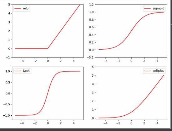
        print(sess.run(var))

激活函数

import tensorflow as tf
import numpy as np
import matplotlib.pyplot as plt

# fake data
x = np.linspace(-5, 5, 200)     # x data, shape=(100, 1)

# following are popular activation functions
y_relu = tf.nn.relu(x)
y_sigmoid = tf.nn.sigmoid(x)
y_tanh = tf.nn.tanh(x)
y_softplus = tf.nn.softplus(x)
# y_softmax = tf.nn.softmax(x)  softmax is a special kind of activation function, it is about probability

sess = tf.Session()
y_relu, y_sigmoid, y_tanh, y_softplus = sess.run([y_relu, y_sigmoid, y_tanh, y_softplus])

# plt to visualize these activation function
plt.figure(1, figsize=(8, 6))
plt.subplot(221)
plt.plot(x, y_relu, c='red', label='relu')
plt.ylim((-1, 5))
plt.legend(loc='best')

plt.subplot(222)
plt.plot(x, y_sigmoid, c='red', label='sigmoid')
plt.ylim((-0.2, 1.2))
plt.legend(loc='best')

plt.subplot(223)
plt.plot(x, y_tanh, c='red', label='tanh')
plt.ylim((-1.2, 1.2))
plt.legend(loc='best')

plt.subplot(224)
plt.plot(x, y_softplus, c='red', label='softplus')
plt.ylim((-0.2, 6))
plt.legend(loc='best')

plt.show()

简单神经网络构造

import tensorflow as tf
import matplotlib.pyplot as plt
import numpy as np

tf.set_random_seed(1)
np.random.seed(1)

# fake data
x = np.linspace(-1, 1, 100)[:, np.newaxis]          # shape (100, 1)
noise = np.random.normal(0, 0.1, size=x.shape)
y = np.power(x, 2) + noise                          # shape (100, 1) + some noise

# plot data
plt.scatter(x, y)
plt.show()

tf_x = tf.placeholder(tf.float32, x.shape)     # input x
tf_y = tf.placeholder(tf.float32, y.shape)     # input y

# neural network layers
l1 = tf.layers.dense(tf_x, 10, tf.nn.relu)          # hidden layer
output = tf.layers.dense(l1, 1)                     # output layer

loss = tf.losses.mean_squared_error(tf_y, output)   # compute cost
optimizer = tf.train.GradientDescentOptimizer(learning_rate=0.5)
train_op = optimizer.minimize(loss)

sess = tf.Session()                                 # control training and others
sess.run(tf.global_variables_initializer())         # initialize var in graph

plt.ion()   # something about plotting 打开交互模式

for step in range(100):
    # train and net output
    _, l, pred = sess.run([train_op, loss, output], {tf_x: x, tf_y: y})
    if step % 5 == 0:
        # plot and show learning process
        plt.cla()#清除活动轴
        plt.scatter(x, y)
        plt.plot(x, pred, 'r-', lw=5)
        plt.text(0.5, 0, 'Loss=%.4f' % l, fontdict={'size': 20, 'color': 'red'})
        plt.pause(0.1)

plt.ioff()#关闭交互模式用于阻塞程序，不让图片关闭
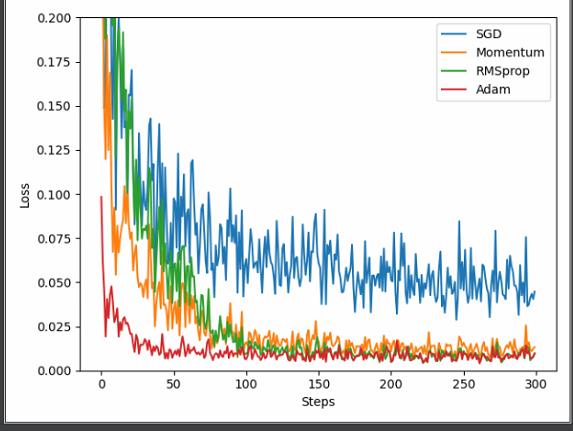
plt.show()

优化器

import tensorflow as tf
import matplotlib.pyplot as plt
import numpy as np

tf.set_random_seed(1)
np.random.seed(1)

LR = 0.01
BATCH_SIZE = 32

# fake data
x = np.linspace(-1, 1, 100)[:, np.newaxis]          # shape (100, 1)
noise = np.random.normal(0, 0.1, size=x.shape)
y = np.power(x, 2) + noise                          # shape (100, 1) + some noise

# plot dataset
plt.scatter(x, y)
plt.show()

# default network
class Net:
    def __init__(self, opt, **kwargs):
        self.x = tf.placeholder(tf.float32, [None, 1])
        self.y = tf.placeholder(tf.float32, [None, 1])
        l = tf.layers.dense(self.x, 20, tf.nn.relu)
        out = tf.layers.dense(l, 1)
        self.loss = tf.losses.mean_squared_error(self.y, out)
        self.train = opt(LR, **kwargs).minimize(self.loss)

# different nets
net_SGD         = Net(tf.train.GradientDescentOptimizer)
net_Momentum    = Net(tf.train.MomentumOptimizer, momentum=0.9)
net_RMSprop     = Net(tf.train.RMSPropOptimizer)
net_Adam        = Net(tf.train.AdamOptimizer)
nets = [net_SGD, net_Momentum, net_RMSprop, net_Adam]

sess = tf.Session()
sess.run(tf.global_variables_initializer())

losses_his = [[], [], [], []]   # record loss

# training
for step in range(300):          # for each training step
    index = np.random.randint(0, x.shape[0], BATCH_SIZE)
    b_x = x[index]
    b_y = y[index]

    for net, l_his in zip(nets, losses_his):
        _, l = sess.run([net.train, net.loss], {net.x: b_x, net.y: b_y})
        l_his.append(l)     # loss recoder

# plot loss history
labels = ['SGD', 'Momentum', 'RMSprop', 'Adam']
for i, l_his in enumerate(losses_his):
    plt.plot(l_his, label=labels[i])
plt.legend(loc='best')
plt.xlabel('Steps')
plt.ylabel('Loss')
plt.ylim((0, 0.2))
plt.show()

 

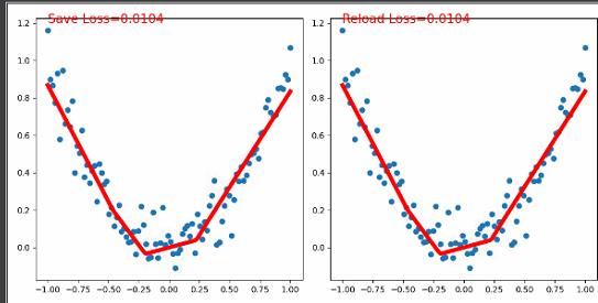
保存模型与加载模型

"""
Know more, visit my Python tutorial page: https://morvanzhou.github.io/tutorials/
My Youtube Channel: https://www.youtube.com/user/MorvanZhou

Dependencies:
tensorflow: 1.1.0
matplotlib
numpy
"""
import tensorflow as tf
import matplotlib.pyplot as plt
import numpy as np

tf.set_random_seed(1)
np.random.seed(1)

# fake data
x = np.linspace(-1, 1, 100)[:, np.newaxis]          # shape (100, 1)
noise = np.random.normal(0, 0.1, size=x.shape)
y = np.power(x, 2) + noise                          # shape (100, 1) + some noise


def save():
    print('This is save')
    # build neural network
    tf_x = tf.placeholder(tf.float32, x.shape)  # input x
    tf_y = tf.placeholder(tf.float32, y.shape)  # input y
    l = tf.layers.dense(tf_x, 10, tf.nn.relu)          # hidden layer
    o = tf.layers.dense(l, 1)                     # output layer
    loss = tf.losses.mean_squared_error(tf_y, o)   # compute cost
    train_op = tf.train.GradientDescentOptimizer(learning_rate=0.5).minimize(loss)

    sess = tf.Session()
    sess.run(tf.global_variables_initializer())  # initialize var in graph

    saver = tf.train.Saver()  # define a saver for saving and restoring

    for step in range(100):                             # train
        sess.run(train_op, {tf_x: x, tf_y: y})

    saver.save(sess, './params', write_meta_graph=False)  # meta_graph is not recommended

    # plotting
    pred, l = sess.run([o, loss], {tf_x: x, tf_y: y})
    plt.figure(1, figsize=(10, 5))
    plt.subplot(121)
    plt.scatter(x, y)
    plt.plot(x, pred, 'r-', lw=5)
    plt.text(-1, 1.2, 'Save Loss=%.4f' % l, fontdict={'size': 15, 'color': 'red'})


def reload():
    print('This is reload')
    # build entire net again and restore
    tf_x = tf.placeholder(tf.float32, x.shape)  # input x
    tf_y = tf.placeholder(tf.float32, y.shape)  # input y
    l_ = tf.layers.dense(tf_x, 10, tf.nn.relu)          # hidden layer
    o_ = tf.layers.dense(l_, 1)                     # output layer
    loss_ = tf.losses.mean_squared_error(tf_y, o_)   # compute cost

    sess = tf.Session()
    # don't need to initialize variables, just restoring trained variables
    saver = tf.train.Saver()  # define a saver for saving and restoring
    saver.restore(sess, './params')

    # plotting
    pred, l = sess.run([o_, loss_], {tf_x: x, tf_y: y})
    plt.subplot(122)
    plt.scatter(x, y)
    plt.plot(x, pred, 'r-', lw=5)
    plt.text(-1, 1.2, 'Reload Loss=%.4f' % l, fontdict={'size': 15, 'color': 'red'})
    plt.show()


save()

# destroy previous net
tf.reset_default_graph()

reload()

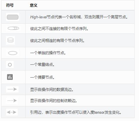
tensorboard可视化

参考文档：TensorBoard:图表可视化 - TensorFlow官方文档中文版 (pythontab.com)

1.创建writer，写日志文件
writer=tf.summary.FileWriter('/path/to/logs', tf.get_default_graph())

2.保存日志文件
writer.close()

3.运行可视化命令，启动服务
tensorboard –logdir /path/to/logs

4.打开可视化界面
通过浏览器打开服务器访问端口http://xxx.xxx.xxx.xxx:6006

TensorBoard的使用流程

1. 添加记录节点：tf.summary.scalar/image/histogram()等
2. 汇总记录节点：merged = tf.summary.merge_all()
3. 运行汇总节点：summary = sess.run(merged)，得到汇总结果
4. 日志书写器实例化：summary_writer = tf.summary.FileWriter(logdir, graph=sess.graph)，实例化的同时传入 graph 将当前计算图写入日志
5. 调用日志书写器实例对象summary_writer的add_summary(summary, global_step=i)方法将所有汇总日志写入文件
6. 调用日志书写器实例对象summary_writer的close()方法写入内存，否则它每隔120s写入一次

"""
Know more, visit my Python tutorial page: https://morvanzhou.github.io/tutorials/
My Youtube Channel: https://www.youtube.com/user/MorvanZhou

Dependencies:
tensorflow: 1.1.0
numpy
"""
import tensorflow as tf
import numpy as np

tf.set_random_seed(1)
np.random.seed(1)

# fake data
x = np.linspace(-1, 1, 100)[:, np.newaxis]          # shape (100, 1)
noise = np.random.normal(0, 0.1, size=x.shape)
y = np.power(x, 2) + noise                          # shape (100, 1) + some noise

with tf.variable_scope('Inputs'):#用tf.variable_scope命名Inputs（名称），x,y属于Inputs层级下的节点
    tf_x = tf.placeholder(tf.float32, x.shape, name='x')
    tf_y = tf.placeholder(tf.float32, y.shape, name='y')

with tf.variable_scope('Net'):
    l1 = tf.layers.dense(tf_x, 10, tf.nn.relu, name='hidden_layer')
    output = tf.layers.dense(l1, 1, name='output_layer')

    # add to histogram summary
    tf.summary.histogram('h_out', l1)
    tf.summary.histogram('pred', output)

loss = tf.losses.mean_squared_error(tf_y, output, scope='loss')
train_op = tf.train.GradientDescentOptimizer(learning_rate=0.5).minimize(loss)
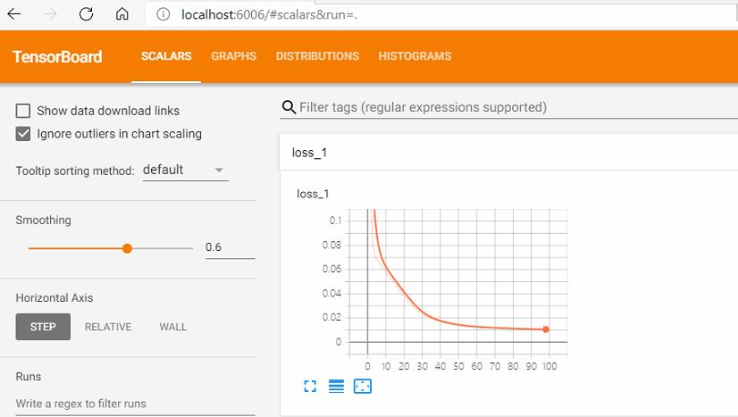
tf.summary.scalar('loss', loss)     # add loss to scalar summary

sess = tf.Session()
sess.run(tf.global_variables_initializer())

writer = tf.summary.FileWriter('./log', sess.graph)     # write to file
merge_op = tf.summary.merge_all()                       # operation to merge all summary

for step in range(100):
    # train and net output
    _, result = sess.run([train_op, merge_op], {tf_x: x, tf_y: y})
    writer.add_summary(result, step)

# Lastly, in your terminal or CMD, type this :
# $ tensorboard --logdir path/to/log
# open you google chrome, type the link shown on your terminal or CMD. (something like this: http://localhost:6006)

注意：节点域：tf2使用tf.name_scope('XX'):使可视化更简洁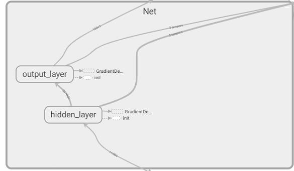

 

启动TensorBoard　

输入下面的指令来启动TensorBoard

tensorboard --logdir=/path/to/log-directory

这里的参数 logdir 指向 SummaryWriter 序列化数据的存储路径。如果logdir目录的子目录中包含另一次运行时的数据，那么 TensorBoard 会展示所有运行的数据。一旦 TensorBoard 开始运行，你可以通过在浏览器中输入 localhost:6006 来查看 TensorBoard。

梯度下降

"""
Know more, visit my Python tutorial page: https://morvanzhou.github.io/tutorials/
My Youtube Channel: https://www.youtube.com/user/MorvanZhou

Dependencies:
tensorflow: 1.1.0
matplotlib
numpy
"""
import tensorflow as tf
import numpy as np
import matplotlib.pyplot as plt
from mpl_toolkits.mplot3d import Axes3D

LR = 0.1
REAL_PARAMS = [1.2, 2.5]
INIT_PARAMS = [[5, 4],
               [5, 1],
               [2, 4.5]][2]

x = np.linspace(-1, 1, 200, dtype=np.float32)   # x data

# Test (1): Visualize a simple linear function with two parameters,
# you can change LR to 1 to see the different pattern in gradient descent.

# y_fun = lambda a, b: a * x + b
# tf_y_fun = lambda a, b: a * x + b


# Test (2): Using Tensorflow as a calibrating tool for empirical formula like following.

# y_fun = lambda a, b: a * x**3 + b * x**2
# tf_y_fun = lambda a, b: a * x**3 + b * x**2


# Test (3): Most simplest two parameters and two layers Neural Net, and their local & global minimum,
# you can try different INIT_PARAMS set to visualize the gradient descent.

y_fun = lambda a, b: np.sin(b*np.cos(a*x))
tf_y_fun = lambda a, b: tf.sin(b*tf.cos(a*x))

noise = np.random.randn(200)/10
y = y_fun(*REAL_PARAMS) + noise         # target

# tensorflow graph
a, b = [tf.Variable(initial_value=p, dtype=tf.float32) for p in INIT_PARAMS]
pred = tf_y_fun(a, b)
mse = tf.reduce_mean(tf.square(y-pred))
train_op = tf.train.GradientDescentOptimizer(LR).minimize(mse)

a_list, b_list, cost_list = [], [], []
with tf.Session() as sess:
    sess.run(tf.global_variables_initializer())
    for t in range(400):
        a_, b_, mse_ = sess.run([a, b, mse])
        a_list.append(a_); b_list.append(b_); cost_list.append(mse_)    # record parameter changes
        result, _ = sess.run([pred, train_op])                          # training


# visualization codes:
print('a=', a_, 'b=', b_)
plt.figure(1)
plt.scatter(x, y, c='b')    # plot data
plt.plot(x, result, 'r-', lw=2)   # plot line fitting
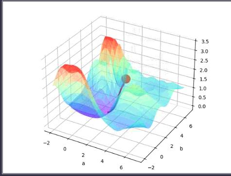
# 3D cost figure
fig = plt.figure(2); ax = Axes3D(fig)
a3D, b3D = np.meshgrid(np.linspace(-2, 7, 30), np.linspace(-2, 7, 30))  # parameter space
cost3D = np.array([np.mean(np.square(y_fun(a_, b_) - y)) for a_, b_ in zip(a3D.flatten(), b3D.flatten())]).reshape(a3D.shape)
ax.plot_surface(a3D, b3D, cost3D, rstride=1, cstride=1, cmap=plt.get_cmap('rainbow'), alpha=0.5)
ax.scatter(a_list[0], b_list[0], zs=cost_list[0], s=300, c='r')  # initial parameter place
ax.set_xlabel('a'); ax.set_ylabel('b')
ax.plot(a_list, b_list, zs=cost_list, zdir='z', c='r', lw=3)    # plot 3D gradient descent
plt.show()