用Python做生存分析--lifelines库简介

Posted 2023-04-07

参考技术A

Python提供了一个简单而强大的生存分析包——lifelines，可以非常方便的进行应用。这篇文章将为大家简单介绍这个包的安装和使用。

lifelines支持用pip的方法进行安装，您可以使用以下命令进行一键安装：

在python中，可以利用lifelines进行累计生存曲线的绘制、Log Rank test、Cox回归等。下面以lifelines包中自带的测试数据进行一个简单的示例。

首先加载和使用自带的数据集：

运行一下将会看到以下结果，

数据有三列，其中T代表min(T, C)，其中T为死亡时间，C为观测截止时间。E代表是否观到“死亡”，1代表观测到了，0代表未观测到，即生存分析中的删失数据，共7个。 group代表是否存在病毒， miR-137代表存在病毒，control代表为不存在即对照组，根据统计，存在miR-137病毒人数34人，不存在129人。

利用此数据取拟合拟生存分析中的Kaplan Meier模型（专用于估计生存函数的模型），并绘制全体人群的生存曲线。

图中蓝色实线为生存曲线，浅蓝色带代表了95%置信区间。随着时间增加，存活概率S(t)越来越小，这是一定的，同时S(t)=0.5时，t的95%置信区间为[53, 58]。这并不是我们关注的重点，我们真正要关注的实验组（存在病毒）和对照组（未存在病毒）的生存曲线差异。因此我们要按照group等于“miR-137”和“control”分组，分别观察对应的生存曲线:

可以看到，带有miR-137病毒的生存曲线在control组下方。说明其平均存活时间明显小于control组。同时带有miR-137病毒存活50%对应的存活时间95%置信区间为[19,29]，对应的control组为[56,60]。差异较大，这个方法可以应用在分析用户流失等场景，比如我们对一组人群实行了一些防止流行活动，我们可以通过此种方式分析我们活动是否有效。

该模型以生存结局和生存时间为应变量，可同时分析众多因素对生存期的影响，能分析带有截尾生存时间的资料，且不要求估计资料的生存分布类型。

对于回归模型的假设检验通常采用似然比检验、Wald检验和记分检验，其检验统计量均服从卡方分布。，其自由度为模型中待检验的自变量个数。一般说来，Cox回归系数的估计和模型的假设检验计算量较大，通常需利用计算机来完成相应的计算

通常存活时间与多种因素都存在关联，因此我们的面临的数据是多维的。下面使用一个更复杂的数据集。首先仍然是导入和使用示例数据。

[图片上传中...(24515569-a5987d05b5e05a26.png-4ed038-1600008755271-0)]

其中T代表min(T, C)，其中T为死亡时间，C为观测截止时间。E代表是否观察到“死亡”，1代表观测到了，0代表未观测到，即生存分析中的 “删失” 数据，删失数据共11个。var1,var2,var3代表了我们关系的变量，可以是是否为实验组的虚拟变量，可以是一个用户的渠道路径，也可以是用户自身的属性。
我们利用此数据进行Cox回归

从结果来看，我们认为var1和var3在5%的显著性水平下是显著的。认为var1水平越高，用户的风险函数值越大，即存活时间越短（cox回归是对风险函数建模，这与死亡加速模型刚好相反，死亡加速模型是对存活时间建模，两个模型的参数符号相反）。同理，var3水平越高，用户的风险函数值越大。

生存分析——跟着lifelines学生存分析建模

笔者看到lifelines的文档里面涵盖的生存分析的模块以及讲解，比能查到的任何地方都要完整，所以 把这个库作为学习素材。
当然，另外也可以参考一下SPSS软件里面的模块，也是非常经典的一些学习对象。

文章目录

• 0 lifelines介绍
• • 0.1 lifelines几个重要方法
  • 0.2 完整的生存分析流程
• 1 生存概率估计
• • 1.1 非参数：KM数据样式——durations
  • 1.2 绘制KM曲线
  • 1.3 分组KM图
  • 1.4 分组KM曲线差异指标
  • • 1.4.1 中位数50%存活率
    • 1.4.2 Logrank检验
  • 1.5 参数估计：生存函数
• 2 Cox 比例风险回归模型
• • 2.1 数据集加载
  • 2.2 比例风险Cox回归
• 3 非比例风险模型——时变风险：Time varying survival regression
• • 3.1 Aalen’s Additive model 模型
  • 3.2 COX风险时变模型：Cox’s time varying proportional hazard model
  • • 3.2.1 数据样式
    • 3.2.2 CoxTimeVaryingFitter 建模
  • 3.3 完整 比例cox -> CoxTimeVarying 探索建模过程
  • • 3.3.1 数据加载
    • 3.3.2 先构建比例COX模型
    • 3.3.3 检验PH假定：proportional_hazard_test
    • 3.3.4 分类变量未沟通PH检验处理方式：strata分层变量
    • 3.3.5 连续变量未沟通PH检验处理方式一：strata分层变量
    • 3.3.6 连续变量未沟通PH检验处理方式二：修改cox公式
    • 3.3.7 连续变量未沟通PH检验处理方式三：分段数据集
  • 3.4 PH检验（proportional hazard assumption）是否一定需要？
• 4 非比例风险模型—— 参数估计模型 Weibull AFT model
• 5 lifelines相关工具函数
• • 5.1 寿命表制作函数——survival_table_from_events
  • 5.2 KM曲线数据样式制作函数
  • 5.3 COX 时变回归模型中的 数据样式制作函数
  • • 5.3.1 第一种：add_covariate_to_timeline
    • 5.3.2 第二种：to_episodic_format
• 6 累计风险函数：Cumulative hazard function
• • 6.1 非参数估计：Nelson-Aalen 累计风险函数图
  • 6.2 参数 估计：其他累计风险参数估计模型
• 7 如何选择最佳的参数估计模型
• • 7.1 QQ图
  • 7.2 AIC图
• 8 其他

---

本系列的续作：

• 生存分析——快手的基于深度学习框架的集成⽣存分析软件KwaiSurvival（一）
• 生存分析——KM生存曲线、hazard比例、PH假定检验、非比例风险模型（分层/时变/参数模型）（二）
• 生存分析——跟着lifelines学生存分析建模（三）

---

0 lifelines介绍

github地址：CamDavidsonPilon/lifelines
文档地址：lifelines

生存分析最初是由精算师和医学界大量开发和应用的。它的目的是回答为什么事件发生在现在，而不是在不确定的情况下(事件可能涉及死亡，疾病缓解等)。
这对那些对测量寿命感兴趣的研究人员来说是件好事:他们可以回答诸如什么因素可能影响死亡之类的问题。但在医学和精算科学之外，还有许多其他有趣和令人兴奋的生存分析应用。
例如:

• SaaS提供商感兴趣的是度量订阅者的生命周期，即首次操作所需的时间
• 库存缺货是对商品真正“需求”的审查事件。
• 社会学家对衡量政党的寿命、关系或婚姻感兴趣
• A/B测试是为了确定不同的团队执行一个动作需要多长时间。

还有用来判断用户流失以及快手有一篇来判定用户活跃度（本质也是从判定流失开始）

0.1 lifelines几个重要方法

在生存分析——KM生存曲线、hazard比例、PH假定检验、非比例风险模型（分层/时变/参数模型）（二）提及到几个，这里笔者自己总结一下lifelines中几个比较核心的：

模块	描述	类型	方法
survival function	研究对象从试验开始直到某个特定时间点仍然存活的概率	参数估计	Exponential, Log-Logistic, Log-Normal and Splines
		非参数估计	Kaplan-Meier估计
cumulative hazard	风险函数的估计值	参数估计	Exponential, Log-Logistic, Log-Normal and Splines
		非参数估计	Nelson-Aalen估计
Survival regression	会加入额外的协变量(如年龄、国家等)与另一个变量进行回归	比例回归	Cox 比例风险回归模型
		非比例回归	含参数与半参模型：Aalen’s Additive model 模型 、 CoxTimeVarying时变模型、AFT(accelerated failure time model)加速失效模型

0.2 完整的生存分析流程

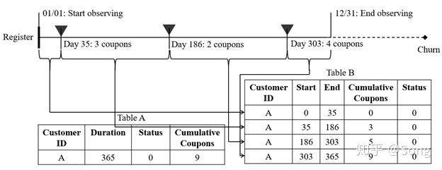
从Time-Dependent 生存模型分析用户流失来看一个完整的生存分析可归纳为：

• 原始数据格式处理：把数据处理为用户、生存时长、是否删失的数据格式。
• KM估计及生存曲线的绘制。
• 判断协变量是否存在时变变量，如果有，进行数据格式的二次处理，将数据打断为用户、起始时间、结束时间、是否删失的格式。
• 判断协变量系数是否存在时变效果，即著名的PH假设检验。如果检验不通过，对时变效果进行绘制，并基于绘制结果进行数据分层（stratify）。
• 建立Extended Cox PH Model，对风险因子进行影响估计。

一个比较好的案例可以参考：【3.3 完整 比例cox -> CoxTimeVarying 探索建模过程】

---

1 生存概率估计

从这篇 数据分析系列：生存分析（生存曲线分析、Cox回归分析）——附生存分析python代码。开始来看一下lifelines实现KM方法，结合lifelines文档，来完整看看KM流程。
生存函数估计有非常多方法：

• 非参估计：Kaplan-Meier
• 参数估计：WeibullFitter等

1.1 非参数：KM数据样式——durations

数据集样式：

from lifelines.datasets import load_waltons
from lifelines import KaplanMeierFitter
from lifelines.utils import median_survival_times
import matplotlib.pyplot as plt

# 数据载入
df = load_waltons()
print(df.head(),'\\n')
print(df['T'].min(), df['T'].max(),'\\n')
print(df['E'].value_counts(),'\\n')
print(df['group'].value_counts(),'\\n')

可以看到数据有三列，其中T代表min(T, C)，其中T为死亡时间，C为观测截止时间。
E代表是否观察到“死亡”，1代表观测到了，0代表未观测到，即生存分析中的删失数据，共7个。
group代表是否存在病毒， miR-137代表存在病毒，control代表为不存在即对照组，根据统计，存在miR-137病毒人数34人，不存在129人。

需要注意，该格式并非严格的寿命表，具体的转化为寿命表可以看[5.1 小节]

1.2 绘制KM曲线

利用此数据取拟合拟生存分析中的Kaplan Meier模型（专用于估计生存函数的模型）

# KM初始化
kmf = KaplanMeierFitter()
kmf.fit(df['T'], event_observed=df['E'])

# 全体: K-M 存活曲线 
kmf.survival_function_  # km 生存概率
kmf.plot_survival_function()

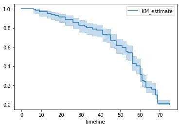
图中蓝色实线为生存曲线，浅蓝色带代表了95%置信区间。
随着时间增加，存活概率S(t)越来越小，这是一定的，同时S(t)=0.5时，t的95%置信区间为[53, 58]。

这里来看几种画法：

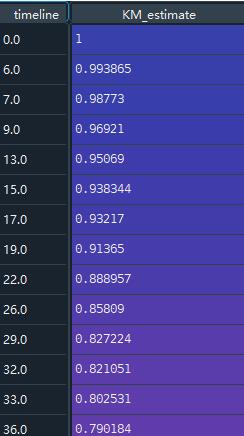
kmf.survival_function_  # km 生存概率
kmf.plot_survival_function()

kmf.survival_function_给出了随着时间增加，KM生存估计概率的趋势。

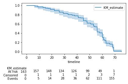
同时还可以在图中画出KM值随着时间上升，原始的删失值以及发生概率：

kmf.plot_survival_function(at_risk_counts=True) # plot_survival_function + 把所有数字也显示出来
plt.tight_layout()

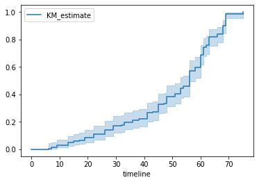
这里还可以画出一条，关于生存概率的，累计概率密度图：

kmf.cumulative_density_   # 累计概率密度图
kmf.plot_cumulative_density() # # 绘制累积密度函数的漂亮图

1.3 分组KM图

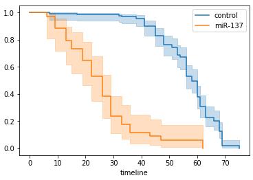
这并不是我们关注的重点，我们真正要关注的实验组（存在病毒）和对照组（未存在病毒）的生存曲线差异。
因此我们要按照group等于“miR-137”和“control”分组，分别观察对应的生存曲线:

# 分组 : K-M 存活曲线
ax = plt.subplot(111)
kmf = KaplanMeierFitter()

for name, grouped_df in df.groupby('group'):
    kmf.fit(grouped_df["T"], grouped_df["E"], label=name)
    kmf.plot_survival_function(ax=ax)

可以看到，带有miR-137病毒的生存曲线在control组下方。说明其平均存活时间明显小于control组。同时带有miR-137病毒存活50%对应的存活时间95%置信区间为[19,29]，对应的control组为[56,60]。

差异较大，这个方法可以应用在分析用户流失等场景，比如我们对一组人群实行了一些防止流行活动，我们可以通过此种方式分析我们活动是否有效。

1.4 分组KM曲线差异指标

除了直接看图，还可以用什么方式来区分不同组的KM曲线：

1.4.1 中位数50%存活率

另外还有中位数50%存活率下存活时间的置信区间：

median_ = kmf.median_survival_time_
median_confidence_interval_ = median_survival_times(kmf.confidence_interval_)
print(median_confidence_interval_) 
>>>     KM_estimate_lower_0.95  KM_estimate_upper_0.95
>>>0.5                    53.0                    58.0

代表着，53-58天左右,存活着整体的一半人。

1.4.2 Logrank检验

Logrank 检验的零假设是指两组的生存时间分布完全一致，当我们通过计算拒绝零假设时，就可以认为两组的生存时间分布存在统计学差异。

from lifelines.statistics import logrank_test

T = df['T']
E = df['E']

dem = (df['group'] == 'miR-137')

results = logrank_test(T[dem], T[~dem], E[dem], E[~dem], alpha=.99)
results.print_summary()
print(results.p_value)
print(results.test_statistic)

输出结果：

<lifelines.StatisticalResult: logrank_test>
               t_0 = -1
 null_distribution = chi squared
degrees_of_freedom = 1
             alpha = 0.99
         test_name = logrank_test

---
 test_statistic      p  -log2(p)
         122.25 <0.005     91.99
2.0359832222854986e-28
122.2491255730062

P值小于0.05 拒绝原假设,存在差异

1.5 参数估计：生存函数

参考：Other parametric models: Exponential, Log-Logistic, Log-Normal and Splines

from lifelines.datasets import load_waltons
from lifelines import KaplanMeierFitter
from lifelines.utils import median_survival_times

# 数据载入
df = load_waltons()
T = df['T']
E = df['E']
print(df.head(),'\\n')
print(df['T'].min(), df['T'].max(),'\\n')
print(df['E'].value_counts(),'\\n')
print(df['group'].value_counts(),'\\n')


import matplotlib.pyplot as plt
import numpy as np
from lifelines import *

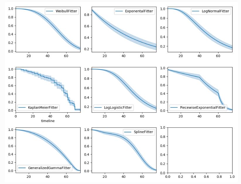
fig, axes = plt.subplots(3, 3, figsize=(13.5, 7.5))

# 多种参数模型
kmf = KaplanMeierFitter().fit(T, E, label='KaplanMeierFitter')
wbf = WeibullFitter().fit(T, E, label='WeibullFitter')
exf = ExponentialFitter().fit(T, E, label='ExponentialFitter')
lnf = LogNormalFitter().fit(T, E, label='LogNormalFitter')
llf = LogLogisticFitter().fit(T, E, label='LogLogisticFitter')
pwf = PiecewiseExponentialFitter([40, 60]).fit(T, E, label='PiecewiseExponentialFitter')
ggf = GeneralizedGammaFitter().fit(T, E, label='GeneralizedGammaFitter')
sf = SplineFitter(np.percentile(T.loc[E.astype(bool)], [0, 50, 100])).fit(T, E, label='SplineFitter')

wbf.plot_survival_function(ax=axes[0][0])
exf.plot_survival_function(ax=axes[0][1])
lnf.plot_survival_function(ax=axes[0][2])
kmf.plot_survival_function(ax=axes[1][0])
llf.plot_survival_function(ax=axes[1][1])
pwf.plot_survival_function(ax=axes[1][2])
ggf.plot_survival_function(ax=axes[2][0])
sf.plot_survival_function(ax=axes[2][1])

---

2 Cox 比例风险回归模型

2.1 数据集加载

与KM的寿命表不太一样，COX是需要协变量的。

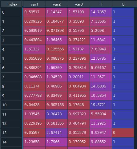
其中T代表min(T, C)，其中T为死亡时间，C为观测截止时间。E代表是否观察到“死亡”，1代表观测到了，0代表未观测到，即生存分析中的**“删失”**数据，删失数据共11个。
var1,var2,var3代表了我们关系的变量，可以是是否为实验组的虚拟变量，可以是一个用户的渠道路径，也可以是用户自身的属性

2.2 比例风险Cox回归

# 模型一初始化 —— Cox proportional hazard model 
cph = CoxPHFitter()
cph.fit(regression_dataset, 'T', event_col='E')
cph.print_summary()

event_col代表事件发生情况，死亡/存活。

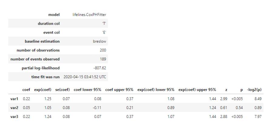
结果分析：从结果来看，我们认为var1和var3在5%的显著性水平下是显著的。认为var1水平越高，用户的风险函数值越大，即存活时间越短（cox回归是对风险函数建模，这与死亡加速模型刚好相反，死亡加速模型是对存活时间建模，两个模型的参数符号相反）。同理，var3水平越高，用户的风险函数值越大。

这里还可以画出每个参数的风险水平coef值：

cph.plot()

---

3 非比例风险模型——时变风险：Time varying survival regression

3.1 Aalen’s Additive model 模型

# 数据加载
from lifelines.datasets import load_regression_dataset
from lifelines import CoxPHFitter
regression_dataset = load_regression_dataset()

print(regression_dataset.head())
print(regression_dataset['E'].value_counts())

# 使用模型 Aalen's Additive model
from lifelines import AalenAdditiveFitter
aaf = AalenAdditiveFitter(fit_intercept=False)
aaf.fit(regression_dataset, 'T', event_col='E')

将$2.2+4.1+3.1$ 的模型一样绘制在图上：

X = regression_dataset.loc[0]

ax = wft.predict_survival_function(X).rename(columns={0:'WeibullAFT'}).plot()
cph.predict_survival_function(X).rename(columns={0:'CoxPHFitter'}).plot(ax=ax)
aaf.predict_survival_function(X).rename(columns={0:'AalenAdditive'}).plot(ax=ax)

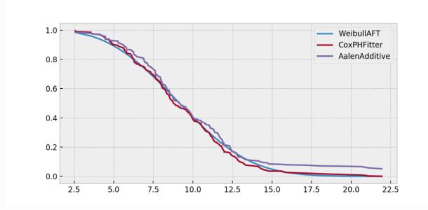
可以观察到三个模型风险预测情况

3.2 COX风险时变模型：Cox’s time varying proportional hazard model

参考：

• Cox’s time varying proportional hazard model
• 生存分析——KM生存曲线、hazard比例、PH假定检验、非比例风险模型（分层/时变/参数模型）（二）

3.2.1 数据样式

一个典型的例子就是多疗程治疗下用户的死亡时间，如果以用户接受的药剂量来做协变量，则属于一个经典时变变量。
因为用户活得越久，接受大疗程越多，注入的要药剂也越多。换而言之，药剂量在用户的生存期内，是随时间变化的，不像性别这些因素一样保持不变。
这样的问题在用户流失中同样存在，如优惠券的累计发放量，同样与药剂量类似。

对于这种变量，我们需要对原始数据做split。根据变化的时间节点，把原始数据打断为多行。

import pandas as pd
from lifelines.utils import to_long_format
from lifelines.utils import add_covariate_to_timeline

base_df = pd.DataFrame([
    {'id': 1, 'duration': 10, 'event': True, 'var1': 0.1},
    {'id': 2, 'duration': 12, 'event': True, 'var1': 0.5}
])
base_df = to_long_format(base_df, duration_col="duration")

cv = pd.DataFrame([
    {'id': 1, 'time': 0, 'var2': 1.4},
    {'id': 1, 'time': 4, 'var2': 1.2},
    {'id': 1, 'time': 8, 'var2': 1.5},
    {'id': 2, 'time': 0, 'var2': 1.6},
])
base_df = add_covariate_to_timeline(base_df, cv, duration_col="time", id_col="id", event_col="event", delay=5)\\
            .fillna(0)

print(base_df)

这里解释一下base_df是基础上的数据，其中ID=1 的事件，经历了10天，然后event发生了，其中var1这里不是时变量。
但是，发现有一个时变变量var2需要给入，而且这个时变量var2，将时间分割为：[[0-4],[4-8],[8-10]]，所以这里通过add_covariate_to_timeline就可以构造这一特殊格式，数据样式输出为：

   start  var1  var2  stop  id  event
0      0   0.1   NaN   5.0   1  False
1      5   0.1   1.4   9.0   1  False
2      9   0.1   1.2  10.0   1   True
3      0   0.5   NaN   5.0   2  False
4      5   0.5   1.6  12.0   2   True

3.2.2 CoxTimeVaryingFitter 建模

from lifelines import CoxTimeVaryingFitter

ctv = CoxTimeVaryingFitter(penalizer=0.1)
ctv.fit(base_df, id_col="id", event_col="event", start_col="start", stop_col="stop", show_progress=True)
ctv.print_summary()
ctv.plot()

输出的内容与之前COX一致：

Iteration 5: norm_delta = 0.00000, step_size = 1.00000, ll = -0.35664, newton_decrement = 0.00000, seconds_since_start = 0.0Convergence completed after 5 iterations.
<lifelines.CoxTimeVaryingFitter: fitted with 5 periods, 2 subjects, 2 events>
         event col = 'event'
         penalizer = 0.1
number of subjects = 2
 number of periods = 5
  number of events = 2
partial log-likelihood = -0.36
  time fit was run = 2021-07-26 06:27:52 UTC

---
            coef  exp(coef)   se(coef)   coef lower 95%   coef upper 95%  exp(coef) lower 95%  exp(coef) upper 95%
covariate                                                                                                         
var1       -3.27       0.04       4.60           -12.28             5.74                 0.00               312.29
var2       -0.26       0.77       1.78            -3.74             3.23                 0.02                25.20

              z    p   -log2(p)
covariate                      
var1      -0.71 0.48       1.07
var2      -0.15 0.88       0.18
---
Partial AIC = 4.71
log-likelihood ratio test = 0.67 on 2 df
-log2(p) of ll-ratio test = 0.49

同时附上ctv.plot()结果：

3.3 完整 比例cox -> CoxTimeVarying 探索建模过程

参考：Testing the proportional hazard assumptions

3.3.1 数据加载

%matplotlib inline
%config InlineBackend.figure_format = 'retina'

from matplotlib import pyplot as plt
from lifelines import CoxPHFitter
import numpy as np
import pandas as pd

rossi = load_rossi()

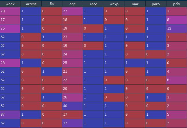
数据集，这里week 代表时间 T ， arrest 代表事件是否发生： event

3.3.2 先构建比例COX模型

cph = CoxPHFitter()
cph.fit(rossi, 'week', 'arrest')  # week = T /  arrest = event
cph.print_summary(model="untransformed variables", decimals=3)

先构建比例COX建模，来进行PH假定

3.3.3 检验PH假定：proportional_hazard_test

有两种方式进行检验：

# 方式一
cph.check_assumptions(rossi, p_value_threshold=0.05, show_plots=True)
 
# 方式二：
from lifelines.statistics import proportional_hazard_test
results = proportional_hazard_test(cph, rossi, time_transform='rank')
results.print_summary(decimals=3, model="untransformed variables")

方式一，这里输出的内容非常多，方拾二类似就不列举了。

输出的第一部分：变量检验表

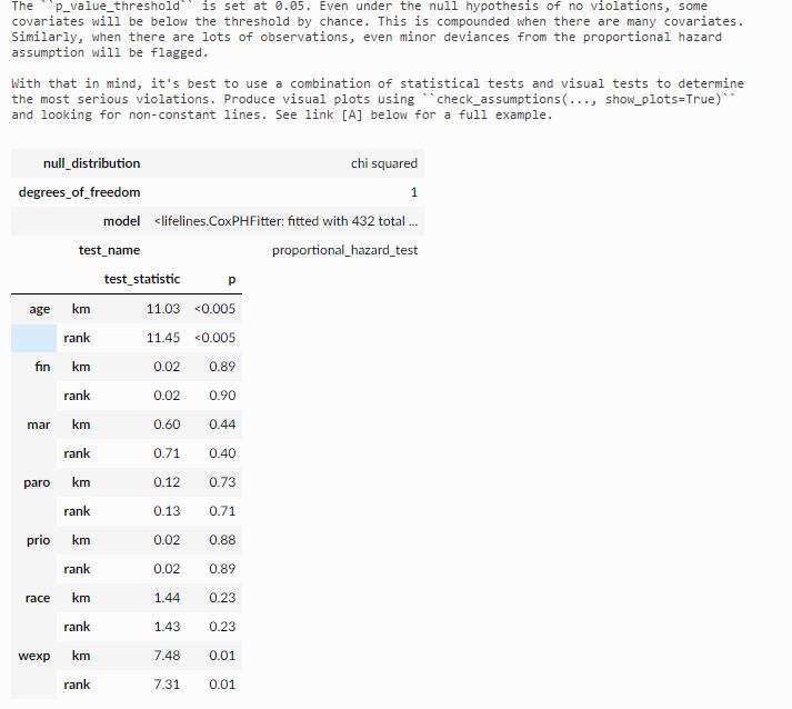
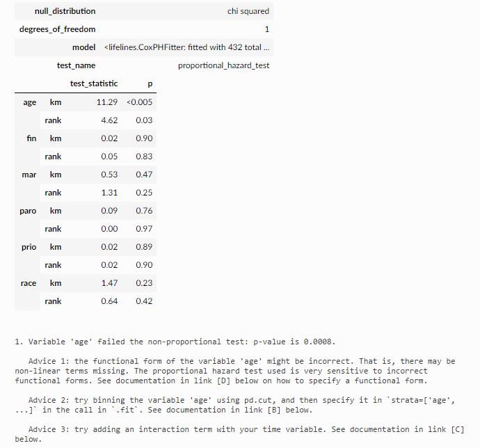
输出结果二：直接指出哪些变量有问题

输出结果三：绘制有问题变量的scaled Schoenfeld residuals

最终结论：
age/wexp p值<0.05 则没有通过假定,协变量相对于基线随时间变化的影响，需要做特殊处理

3.3.4 分类变量未沟通PH检验处理方式：strata分层变量

wexp 没有通过proportional假定,而且wexp分类变量,适合作为strata分层变量
这里不通过假定,可能是因为,样本里面不同分组的差异非常大,变量 -> 时间改变，
我们可以根据某些变量(我们称之为strata分层变量)将数据集划分为子样本，对所有子样本运行Cox模型，并比较它们的差异

cph.fit(rossi, 'week', 'arrest', strata=['wexp'])
cph.print_summary(model="wexp in strata")

将wexp变为strata分层变量之后，再进行ph检验：

cph.check_assumptions(rossi, show_plots=True)

发现wexp 已经检验通过，但是age还不行

3.3.5 连续变量未沟通PH检验处理方式一：strata分层变量

那么这里第一种方式还是把age变量分箱pd.cut，然后进行分层：

# age修复二:age进行分层 并作为分层变量 与wexp一致的做法
rossi_strata_age = rossi.copy()
rossi_strata_age['age_strata'] = pd.cut(rossi_strata_age['age'], np.arange(0, 80, 3))

rossi_strata_age[['age', 'age_strata']].head()

rossi_strata_age = rossi_strata_age.drop('age', axis=1)
cph.fit(rossi_strata_age, 'week', 'arrest', strata=['age_strata', 'wexp'])

cph.print_summary(3, model="stratified age and wexp")
cph.plot()

cph.check_assumptions(rossi_strata_age)
>>> Proportional hazard assumption looks okay.

这里有一个问题就是，分箱越细，那么结论越精准，分箱越粗，结论就会有信息损失在分箱过程中。
这是一个需要平衡的问题。
最终检验，此时全部通过了检验。

3.3.6 连续变量未沟通PH检验处理方式二：修改cox公式

直接贴原文好了：

The proportional hazard test is very sensitive (i.e. lots of false positives) when the functional form of a variable is incorrect. For example, if the association between a covariate and the log-hazard is non-linear, but the model has only a linear term included, then the proportional hazard test can raise a false positive.

这里可以看到需要探索各类非线性age~log-hazard 是否可行：

# age修复一:修改cox公式
rossi['age**2'] = (rossi['age'] - rossi['age'].mean())**2
rossi['age**3'] = (rossi['age'] - rossi['age'].mean())**3


cph.fit(rossi, 'week', 'arrest', strata=['wexp'], formula="bs(age, df=4, lower_bound=10, upper_bound=50) + fin +race + mar + paro + prio")
cph.print_summary(model="spline_model"); print()
cph.check_assumptions(rossi, show_plots=True, p_value_threshold=0.05)

这里可以看到如果加入一些非线性age的形态，wexp之前造成的PH干扰也在减小，
所以通常来说，改变公式形态，都会对其他变量产生有利影响，此时我们甚至可以移除作为分层变量的wexp（strata=['wexp']）

3.3.7 连续变量未沟通PH检验处理方式三：分段数据集

age修复三:Introduce time-varying covariates : 整改数据源，再次依据age进行时变整合

• 第一步：转换成episodic格式
• 第二步：在年龄和stop时间节点上,构造一个时间交互变量
• 之后：使用TimeVaryingFitter进行分析

from lifelines.utils import to_episodic_format

# the time_gaps parameter specifies how large or small you want the periods to be.
rossi_long = to_episodic_format(rossi, duration_col='week', event_col='arrest', time_gaps=1.)
rossi_long.head(25)

rossi_long['time*age'] = rossi_long['age'] * rossi_long['stop']

from lifelines import CoxTimeVaryingFitter
ctv = CoxTimeVaryingFitter()

ctv.fit(rossi_long,
        id_col='id',
        event_col='arrest',
        start_col='start',
        stop_col='stop',
        strata=['wexp'])

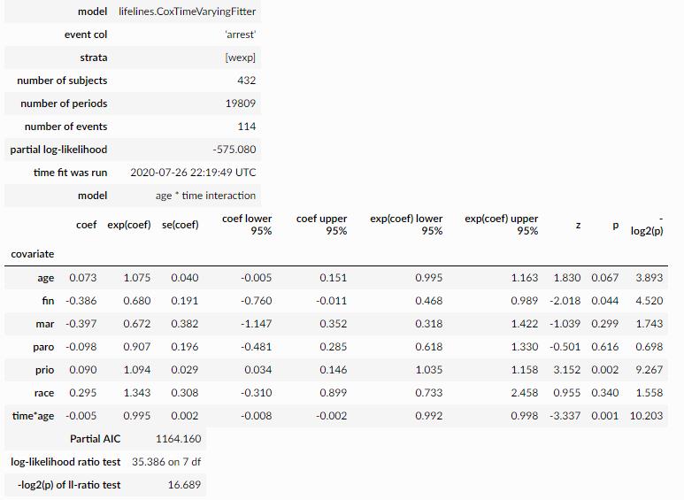
ctv.print_summary(3, model="age * time interaction")

ctv.plot()

先来看一下to_episodic_format是一个什么操作：

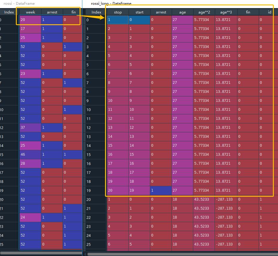
之前某一条记录week = 20，那么现在拆分成20条记录，逐条记录，从start -> stop，其余协变量在20记录中保持不变。
然后这里rossi_long['time*age'] = rossi_long['age'] * rossi_long['stop']是一步非常有意思的操作，就是将age构造成随时间变化的time-varying variable了
最后使用CoxTimeVaryingFitter进行cox回归检验

来看一下scaled Schoenfeld 残差图：

ctv.plot()

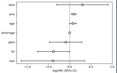
在以上年龄的Schoenfeld残差图中，我们可以看到，时间值越大，风险为正，则有轻微的负效应。
这在coxtimevariyingfitter的输出中得到了证实:我们看到时间*年龄的系数是-0.005。

3.4 PH检验（proportional hazard assumption）是否一定需要？

参考：Do I need to care about the proportional hazard assumption?
是否需要时变检验？以下情况可以忽略：

• 如果你在意生存预测，那么风险的假定可以忽略
• 足够多的样本量，存在一定假定问题是正常的现象
• 有合理的理由假设所有的数据集都会违反比例风险假设【参考： Stensrud & Hernán’s “Why Test for Proportional Hazards?】

4 非比例风险模型—— 参数估计模型 Weibull AFT model

AFT(accelerated failure time model)加速失效模型

AFT模型可见文档：the-log-normal-and-log-logistic-aft-models
模型详细解释：WeibullAFTFitter

与比例COX的例子一样的数据集，来看一下Weibull AFT model：

from lifelines.datasets import load_regression_dataset
from lifelines import CoxPHFitter

regression_dataset = load_regression_dataset()
print(regression_dataset.head())
print(regression_dataset['E'].value_counts())

# 模型二初始化 —— Weibull accelerated failure time model
from lifelines import WeibullAFTFitter

wft = WeibullAFTFitter()
wft.fit(regression_dataset, 'T', event_col='E')
wft.print_summary()
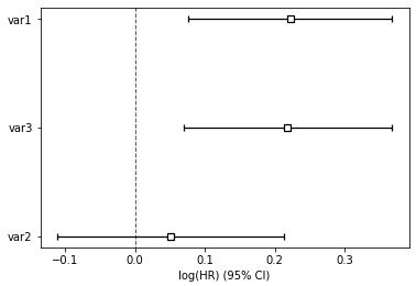
wft.plot()

结果展示：

"""
<lifelines.WeibullAFTFitter: fitted with 200 total observations, 11 right-censored observations>
             duration col = 'T'
                event col = 'E'
   number of observations = 200
number of events observed = 189
           log-likelihood = -504.48
         time fit was run = 2020-06-21 12:27:05 UTC

---
                     coef  exp(coef)   se(coef)   coef lower 95%   coef upper 95%  exp(coef) lower 95%  exp(coef) upper 95%
lambda_ var1        -0.08       0.92       0.02            -0.13            -0.04                 0.88                 0.97
        var2        -0.02       0.98       0.03            -0.07             0.04                 0.93                 1.04
        var3        -0.08       0.92       0.02            -0.13            -0.03                 0.88                 0.97
        Intercept   2.53      12.57       0.05             2.43             2.63                11.41                13.85
rho_    Intercept   1.09       2.98       0.05             0.99             1.20                 2.68                 3.32

                       z      p   -log2(p)
lambda_ var1       -3.45 <0.005      10.78
        var2       -0.56   0.57       0.80
        var3       -3.33 <0.005      10.15
        Intercept 51.12 <0.005        inf
rho_    Intercept 20.12 <0.005     296.66
---
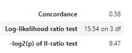
Concordance = 0.58
AIC = 1018.97
log-likelihood ratio test = 19.73 on 3 df
-log2(p) of ll-ratio test = 12.34
"""

最后画图：

---

5 lifelines相关工具函数

5.1 寿命表制作函数——survival_table_from_events

我们在1.1 小节看到KM的数据格式为：

from lifelines.datasets import load_waltons
from lifelines import KaplanMeierFitter
from lifelines.utils import median_survival_times
import matplotlib.pyplot as plt

# 数据载入
df = load_waltons()
print(df.head(),'\\n')
print(df['T'].min(), df['T'].max(),'\\n')
print(df['E'].value_counts(),'\\n')
print(df['group'].value_counts(),'\\n')

这里并非严格的寿命表的数据样式，这里lifelines可以有函数进行转化：

# Perhaps you are interested in viewing the survival table given some durations and censoring vectors.
from lifelines.utils import survival_table_from_events
df = load_waltons()
T = df['T']
E = df['E']

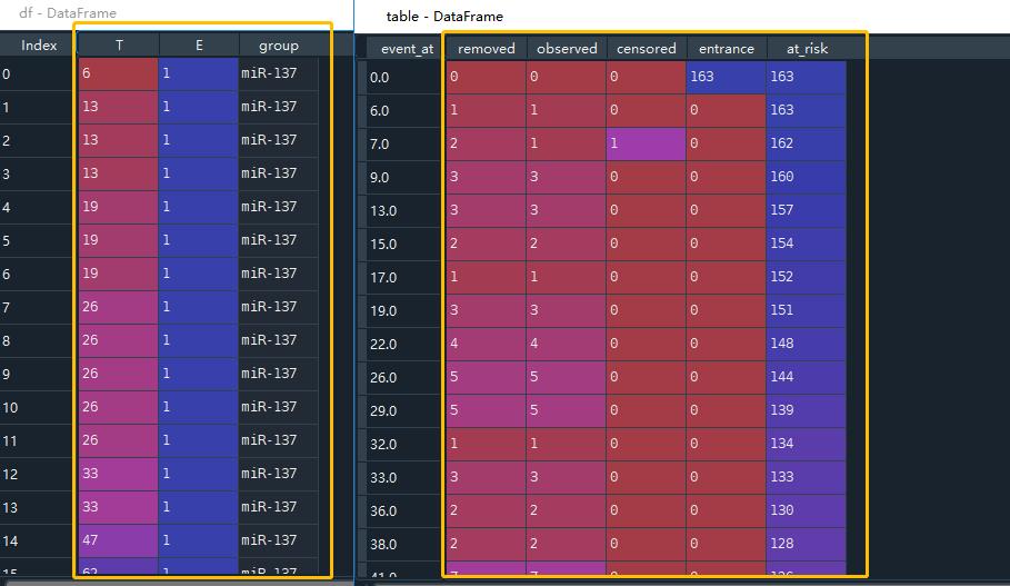
table = survival_table_from_events(T, E)
print(table.head())

进行survival_table_from_events可以变为寿命表的样式。

5.2 KM曲线数据样式制作函数

来看lifelines专门制作KM曲线数据集的函数，也就是刚刚贴的：

from lifelines.utils import datetimes_to_durations

start_dates = ['2015-01-01', '2015-04-01', '2014-04-05']
end_dates = ['2016-02-02', None, '2014-05-06']

T, E = datetimes_to_durations(start_dates, end_dates, freq="D")

>>> T # array([ 397., 1414.,   31.])
>>> E # array([ True, False,  True])

比如这里有三个样本，开始时间为：['2015-01-01', '2015-04-01', '2014-04-05']，
其中有两个在观测期结束了，还有一个没有结束，那么就是['2016-02-02', None, '2014-05-06']
最后给出的数据，T就是结束 - 开始 的durations
E就是最终事件是否发生的event

5.3 COX 时变回归模型中的 数据样式制作函数

5.3.1 第一种：add_covariate_to_timeline

这里其实在3.2.1 已经提及了一种，就复制一下：

import pandas as pd
from lifelines.utils import to_long_format
from lifelines.utils import add_covariate_to_timeline

base_df = pd.DataFrame([
    {'id': 1, 'duration': 10, 'event': True, 'var1': 0.1},
    {'id': 2, 'duration': 12, 'event': True, 'var1': 0.5}
])
base_df = to_long_format(base_df, duration_col="duration")

cv = pd.DataFrame([
    {'id': 1, 'time': 0, 'var2': 1.4},
    {'id': 1, 'time': 4, 'var2': 1.2},
    {'id': 1, 'time': 8, 'var2': 1.5},
    {'id': 2, 'time': 0, 'var2': 1.6},
])
base_df = add_covariate_to_timeline(base_df, cv, duration_col="time", id_col="id", event_col="event", delay=5)\\
            .fillna(0)

print(base_df)

base_df 相当于没有时变协变量的情况下的数据样本，
cv是有时变协变量的数据样本，
最后两者拼接在一些

5.3.2 第二种：to_episodic_format

第二种就是在3.3.7中提及的发现某一连续变量age需要改成时变，然后通过to_episodic_format变为逐条。
同时，需要 age变量*stoptime 构造成为随时间变化的变量

from lifelines.utils import to_episodic_format

# the time_gaps parameter specifies how large or small you want the periods to be.
rossi_long = to_episodic_format(rossi, duration_col='week', event_col='arrest', time_gaps=1.)
rossi_long.head(25)

rossi_long['time*age'] = rossi_long['age'] * rossi_long['stop']

from lifelines import CoxTimeVaryingFitter
ctv = CoxTimeVaryingFitter()

ctv.fit(rossi_long,
        id_col='id',
        event_col='arrest',
        start_col='start',
        stop_col='stop',
        strata=['wexp'])

ctv.print_summary(3, model="age * time interaction")

ctv.plot()

6 累计风险函数：Cumulative hazard function

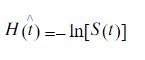
The cumulative hazard has less obvious understanding than the survival functions, but the hazard functions is the basis of more advanced techniques in survival analysis. Recall that we are estimating cumulative hazard functions, H(t). (Why? The sum of estimates is much more stable than the point-wise estimates.) Thus we know the rate of change of this curve is an estimate of the hazard function.

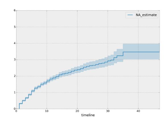
6.1 非参数估计：Nelson-Aalen 累计风险函数图

参考：生存分析论文
在有删失的情况下，可以根据累积死亡率与生存函数的关系，来估计累计风险函数图

也可以参考之前文章中的：2.3 生存/风险函数 两者之间关系
其与与以KM估计式为基础的估计式相比，具有更好的小样本性质，由Nelson提出然后Aalen加以改进

主要作用有：

• 选择事件发生时间的参数模型方面的应用
• 其二是为死亡率h(t)提供粗估计

在lifelines中的实现：

from lifelines.datasets import load_dd

data = load_dd()
data.head()

T = data["duration"]
E = data["observed"]

from lifelines import NelsonAalenFitter
naf = NelsonAalenFitter()

naf.fit(T,event_observed=E)


print(naf.cumulative_hazard_.head())
naf.plot_cumulative_hazard()

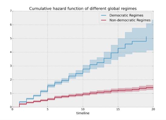
分组来看不同group的累计风险概率：

dem = (data["democracy"] == "Democracy")

naf.fit(T[dem], event_observed=E[dem], label="Democratic Regimes")
ax = naf.plot_cumulative_hazard(loc=slice(0, 20))

naf.fit(T[~dem], event_observed=E[~dem], label="Non-democratic Regimes")
naf.plot_cumulative_hazard(ax=ax, loc=slice(0, 20))

plt.title("Cumulative hazard function of different global regimes");

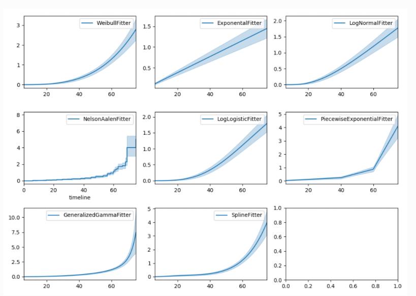
6.2 参数 估计：其他累计风险参数估计模型

与1.5一致，累计风险函数图和生存函数的估计，都有非参数以及参数估计的两种：

参考：Other parametric models: Exponential, Log-Logistic, Log-Normal and Splines

from lifelines import (WeibullFitter, ExponentialFitter,
LogNormalFitter, LogLogisticFitter, NelsonAalenFitter,
PiecewiseExponentialFitter, GeneralizedGammaFitter, SplineFitter)

from lifelines.datasets import load_waltons
data = load_waltons()

fig, axes = plt.subplots(3, 3, figsize=(10, 7.5))

T = data['T']
E = data['E']

wbf = WeibullFitter().fit(T, E, label='WeibullFitter')
exf = ExponentialFitter().fit(T, E, label='ExponentialFitter')
lnf = LogNormalFitter().fit(T, E, label='LogNormalFitter')
naf = NelsonAalenFitter().fit(T, E, label='NelsonAalenFitter')
llf = LogLogisticFitter().fit(T, E, label='LogLogisticFitter')
pwf = PiecewiseExponentialFitter([40, 60]).fit(T, E, label='PiecewiseExponentialFitter')
gg = GeneralizedGammaFitter().fit(T, E, label='GeneralizedGammaFitter')
spf = SplineFitter([6, 20, 40, 75]).fit(T, E, label='SplineFitter')

wbf.plot_cumulative_hazard(ax=axes[0][0])
exf.plot_cumulative_hazard(ax=axes[0][1])
lnf.plot_cumulative_hazard(ax=axes[0][2])
naf.plot_cumulative_hazard(ax=axes[1][0])
llf.plot_cumulative_hazard(ax=axes[1][1])
pwf.plot_cumulative_hazard(ax=axes[1][2])
gg.plot_cumulative_hazard(ax=axes[2][0])
spf.plot_cumulative_hazard(ax=axes[2][1])

7 如何选择最佳的参数估计模型

从第一节和第六节来看，生存函数 以及 累计风险函数都有参数估计以及非参数估计，
参数估计也有非常多的分布可以选择，那么如何哪一种是最好的呢？

lifelines 提供了两种：

• qq-plots QQ图： Selecting a parametric model using QQ plots
• AIC对比图：Selecting a parametric model using AIC

7.1 QQ图

from lifelines import *

from lifelines.plotting import qq_plot

# generate some fake log-normal data
N = 1000
T_actual = np.exp(np.random.randn(N))
C = np.exp(np.random.randn(N))
E = T_actual < C
T = np.minimum(T_actual, C)

fig, axes = plt.subplots(2, 2, figsize=(8, 6))
axes = axes.reshape(4,)

for i, model in enumerate([WeibullFitter(), LogNormalFitter(), LogLogisticFitter(), ExponentialFitter()]):
    model.fit(T, E)
    qq_plot(model, ax=axes[i])

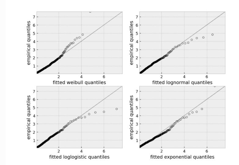
这个图形测试可以用来使模型失效。
例如，在上图中，我们可以看到只有对数正态(log-normal)参数模型是合适的(我们预计尾部会有偏差，但不会太多)。

7.2 AIC图

from lifelines.utils import find_best_parametric_model
from lifelines.datasets import load_lymph_node

T = load_lymph_node()['rectime']
E = load_lymph_node()['censrec']

best_model, best_aic_ = find_best_parametric_model(T, E, scoring_method="AIC")

print(best_model)
# <lifelines.SplineFitter:"Spline_estimate", fitted with 686 total observations, 387 right-censored observations>

best_model.plot_hazard()

这里输出结果的时候会有提示，也就是比较好的是SplineFitter估计：

# <lifelines.SplineFitter:"Spline_estimate", fitted with 686 total observations, 387 right-censored observations>

8 其他

学不废了，这个库还有很多高阶的可以学习的，本篇就到这了。。
还有：

• Piecewise exponential models and creating custom models
  分段指数模型以及可以自定义一些生存函数
• Time-lagged conversion rates and cure models
  譬如犯罪，有的犯罪的人第二次基本不会再犯了，那么就是长期生存者or治愈者，在充分的随访时间中，这些人不过发生某一特定事件，有非常长的截尾时间；
  如果继续使用参数估计会有造成问题：

There’s a serious fault in using parametric models for these types of problems that non-parametric models don’t have. The most common parametric models like Weibull, Log-Normal, etc. all have strictly increasing cumulative hazard functions, which means the corresponding survival function will always converge to 0.