统计学习笔记 线性回归
Posted 知海无涯学无止境
tags:
篇首语:本文由小常识网(cha138.com)小编为大家整理,主要介绍了统计学习笔记 线性回归相关的知识,希望对你有一定的参考价值。
Basic Introduction
In this chapter, we review some of the key ideas underlying the linear regression model, as well as the least squares approach that is most commonly used to fit this model.
Basic form:
![]()
“≈” means “is approximately modeled as”, to estimate the parameters, by far the most common approach involves minimizing the least squares criterion. Let training samples be (x1,y1),...,(xn,yn), then define the residual sum of squares (RSS) as
![]()
And we get
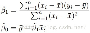
About the result, in the ideal case, that is with enough samples, we can get a classification result called population regression line.
Population regression line: the best fitting result
Least squared regression line: with limited samples
To evaluatehow well our estimation meets the true values, we use standard error, e.g. to estimate the mean value. The variance of sample mean  is
is
![]()
where σ is the standard deviation of each of the realization yi (i=1,2,...,n, y1,...yn are uncorrelated). n is the number of samples.
Definition of standard deviation:
Suppose X is a random variable with mean value

It is the square root of variance. About the computation of standard deviation:
Let x1, ..., xN be samples, then we calculate the standard deviation with (here is the number of limited samples):
![]()
Note: for limited samples, we use N-1 to divide, which is the common case, for unlimited samples in the ideal case, we use N to divide.
In the following formulation:
![]()
![]() ,
,![]()
Here SE means standard error. Standard error is standard deviation divided by sqrt(n), it means the accuracy of results while the standard deviation means the accuracy of data.
An estimation of σ is residual standard error. We use residual standard error (RSE) to estimate it.
![]()
The 95% confidence interval for β1 and β0:
![]()
![]()
As an example, we can use

to get the probability that β1 is zero, or the non-existence of the relationship between X(predictor) and Y(response).
Assessing the Accuracy of the Model
There are 3 criterions:
1. Residual Standard Error


2. R^2 Statistic
![]()
![]()
TSS measures the total variance in the response Y, and can be thought of as the amount of variability inherent in the response before the regression is performed. In contrast, RSS measures the amount of variability that is left unexplained after performing the regression. TSS − RSS measures the amount of variability in the response that is explained (or removed) by performing the regression. An R^2 statistic that is close to 1 indicates that a large proportion of the variability in the response has been explained by the regression. On the other hand, we can use

to assess the fit of the linear model. In simple linear model,R^2=Cor(X,Y)^2.
R^2 is normalized, when the actual line is steeper, TSS is larger, and because of

RSS is also larger.
Multiple Linear Regression
![]()
we can use least squares to get

we also use F-statistic to

An explanation of the above expression is
![]()
![]()
The RSS represents the variability left unexplained, TSS is the total variability, as we have already estimated p variables and there are n variables as a whole, so the variance of RSS is n-p-1, TSS-RSS is p.
Subtopic0: Hypothesis Testing in Single and Multiple Linear Regression
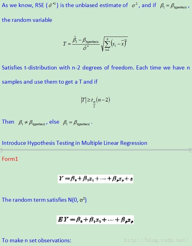
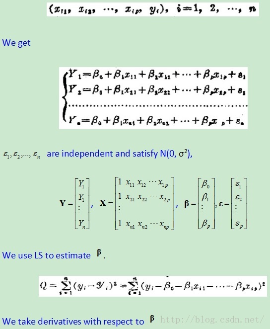

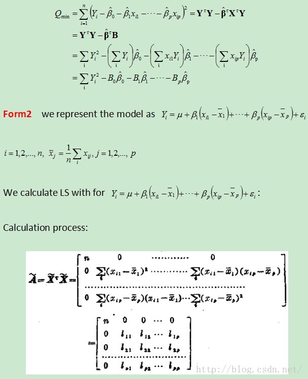
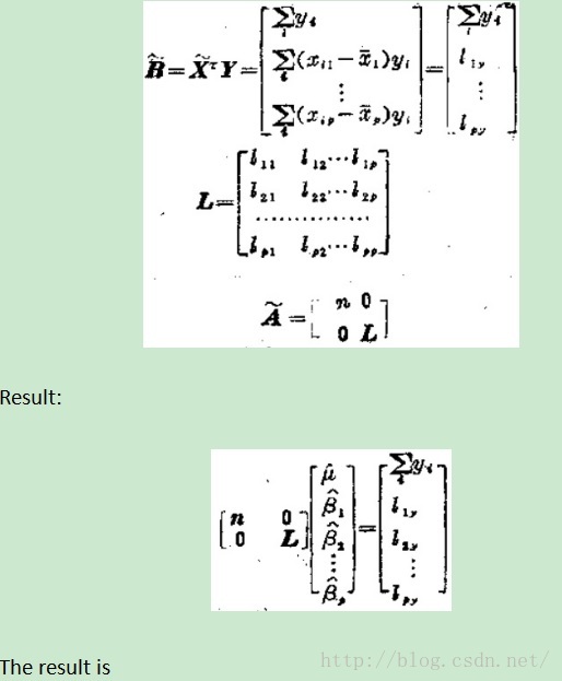

The zero in Q剩 should be changed to 1.

Subtopic1:whether each of the predictors is useful in predicting the response.
To indicate which one of
![]()

is true. If F-statistic is close to 1, then H0 is true. If F-statistic is greater than 1, then Ha is true.
It turns out that the answer depends on the values of n and p. When n is large, an F-statistic that is just a little larger than 1 might still provide evidence against H0. In contrast, a larger F-statistic is needed to reject H0 if n is small.
When H0 is true and the errors i have a normal distribution, the F-statistic follows an F-distribution. For any given value of n and p, any statistical software package can be used to compute the p-value associated with the F-statistic using this distribution. Based on this p-value, we can determine whether or not to reject H0.
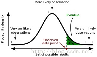
Here the p-value is defined as the probability, under the assumption of hypothesis H, of obtaining a result equal to or more extreme than what was actually observed. Here the reason that a smaller p can indicate the existence of the relationship between at least one of p parameters and the result is that onlyWhen H0 is true and the errors i have a normal distribution, the F-statistic follows an F-distribution. And when p is small, the hypothesis under consideration may not adequately explain the observation.The smaller p-value is, the more suspectable H0 is.
以上是关于统计学习笔记 线性回归的主要内容,如果未能解决你的问题,请参考以下文章