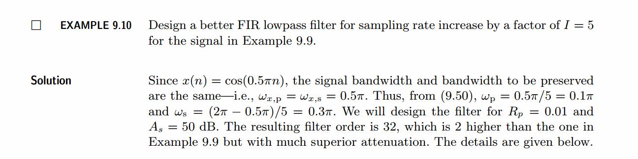
《DSP using MATLAB》示例 Example 9.10

Posted 2020-09-20 沧海一粟

代码：

%% ------------------------------------------------------------------------
%%            Output Info about this m-file
fprintf(\'\\n***********************************************************\\n\');
fprintf(\'        <DSP using MATLAB> Exameple 9.10 \\n\\n\');

time_stamp = datestr(now, 31);
[wkd1, wkd2] = weekday(today, \'long\');
fprintf(\'      Now is %20s, and it is %7s  \\n\\n\', time_stamp, wkd2);
%% ------------------------------------------------------------------------

% Given parameters:
n = [0:50]; wxp = 0.5*pi; x = cos(wxp*n);
n1 = n(1:9); x1 = x(9:17);             % for plotting purposes

I = 5; Rp = 0.01; As = 50; wp = wxp/I; ws = (2*pi-wxp)/I; 
[delta1, delta2] = db2delta(Rp, As); weights = [delta2/delta1, 1];
[N, Fo, Ao, weights] = firpmord([wp, ws]/pi, [1, 0], [delta1, delta2], 2); N = N + 2;
N

%% -----------------------------------------------------------------
%%                             Plot
%% -----------------------------------------------------------------  

% Input signal
Hf1 = figure(\'units\', \'inches\', \'position\', [1, 1, 8, 6], ...
	\'paperunits\', \'inches\', \'paperposition\', [0, 0, 6, 4], ...
	\'NumberTitle\', \'off\', \'Name\', \'Exameple 9.10\');
set(gcf,\'Color\',\'white\'); 

TF = 10;

subplot(2, 2, 1); 
Hs1 = stem(n1, x1, \'filled\'); set(Hs1, \'markersize\', 2, \'color\', \'g\');
axis([-1, 9, -1.2, 1.2]); grid on;
xlabel(\'n\', \'vertical\', \'middle\'); ylabel(\'Amplitude\'); 
title(\'Input Signal x(n)\', \'fontsize\', TF);
set(gca, \'xtick\', [0:4:16]); 
set(gca, \'ytick\', [-1, 0, 1]);


% Interpolation with Filter Design: Length M=31
%M = 31; F = [0, wp, ws, pi]/pi; A = [I, I, 0, 0];
h = firpm(N, Fo, I*Ao, weights); y = upfirdn(x, h, I);
delay = (N)/2;                                                   % Delay imparted by the filter
m = delay+1:1:50*I+delay+1; y = y(m); m = 0:40; y = y(81:121);   % for plotting


subplot(2, 2, 3); 
Hs2 = stem(m, y, \'filled\'); axis([-5, 45, -1.2, 1.2]); grid on;
set(Hs2, \'markersize\', 2, \'color\', \'m\');
xlabel(\'m\', \'vertical\', \'middle\'); ylabel(\'Amplitude\'); 
title(\' Output Singal y(n): I = 5\', \'fontsize\', TF);
set(gca, \'xtick\', [0:4:16]*I); 
set(gca, \'ytick\', [-1, 0, 1]);


% Filter Desing Plots
[Hr, w, a, L] = Hr_Type1(h); Hr_min = min(Hr); w_min = find(Hr == Hr_min);
H = abs(freqz(h, 1, w)); Hdb = 20*log10(H/max(H)); min_attn = Hdb(w_min);

subplot(2, 2, 2);
plot(w/pi, Hr, \'m\', \'linewidth\', 1.0); axis([0, 1, -1, 6]); grid on;
xlabel(\'Frequency in \\pi units\', \'vertical\', \'middle\'); ylabel(\'Amplitude\'); 
title(\'Amplitude Response \', \'fontsize\', TF);
set(gca, \'xtick\', [0, wp/pi, ws/pi, 1]); 
set(gca, \'ytick\', [0, I]);

subplot(2, 2, 4); 
plot(w/pi, Hdb, \'m\', \'linewidth\', 1.0); axis([0, 1, -70, 10]); grid on;
xlabel(\'Frequency in \\pi units\', \'vertical\', \'middle\'); ylabel(\'Decibels\'); 
title(\'Log-magnitude Response \', \'fontsize\', TF);
set(gca, \'xtick\', [0, wp/pi, ws/pi, 1]); 
set(gca, \'ytick\', [-70, round(min_attn), 0]);

　　运行结果：

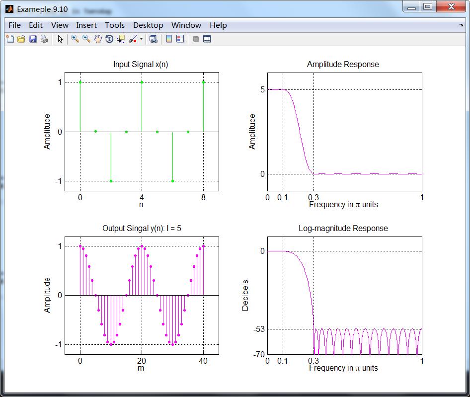
        设计的滤波器最小阻带衰减为53dB。