《DSP using MATLAB》示例Example 8.24

Posted 2020-09-12 沧海一粟

代码：

%% ------------------------------------------------------------------------
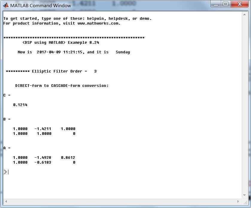
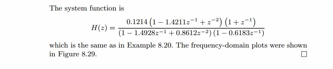
%%            Output Info about this m-file
fprintf(\'\\n***********************************************************\\n\');
fprintf(\'        <DSP using MATLAB> Exameple 8.24 \\n\\n\');

time_stamp = datestr(now, 31);
[wkd1, wkd2] = weekday(today, \'long\');
fprintf(\'      Now is %20s, and it is %8s  \\n\\n\', time_stamp, wkd2);
%% ------------------------------------------------------------------------

% Digital Filter Specifications:
wp = 0.2*pi;                 % digital passband freq in rad
ws = 0.3*pi;                 % digital stopband freq in rad
Rp = 1;                      % passband ripple in dB
As = 15;                     % stopband attenuation in dB

% Analog prototype specifications: Inverse Mapping for frequencies
T = 1;                           % set T = 1
OmegaP = (2/T)*tan(wp/2);        % Prewarp(Cutoff) prototype passband freq
OmegaS = (2/T)*tan(ws/2);        % Prewarp(cutoff) prototype stopband freq

% Analog Elliptic Prototype Order Calculations:
ep = sqrt(10^(Rp/10)-1);           % Passband Ripple Factor
A = 10^(As/20);                    % Stopband Attenuation Factor
OmegaC = OmegaP;                   % Analog Elliptic prototype cutoff freq
k = OmegaP/OmegaS;                 % Analog prototype Transition ratio
k1 = ep/sqrt(A*A-1);               % Analog prototype Intermediate cal
capk = ellipke([k.^2 1-k.^2]);
capk1 = ellipke([(k1 .^2) 1-(k1 .^2)]);

N  = ceil(capk(1)*capk1(2)/(capk(2)*capk1(1)));
fprintf(\'\\n\\n ********** Elliptic Filter Order = %3.0f  \\n\', N)

% Digital Chebyshev-2 Filter Design:
wn = wp/pi;                        % Digital cutoff freq in pi units

[b, a] = ellip(N, Rp, As, wn); [C, B, A] = dir2cas(b, a)

% Calculation of Frequency Response:
[db, mag, pha, grd, ww] = freqz_m(b, a);


%% -----------------------------------------------------------------
%%                             Plot
%% -----------------------------------------------------------------  

figure(\'NumberTitle\', \'off\', \'Name\', \'Exameple 8.24\')
set(gcf,\'Color\',\'white\'); 
M = 1;                          % Omega max

subplot(2,2,1); plot(ww/pi, mag); axis([0, M, 0, 1.2]); grid on;
xlabel(\' frequency in \\pi units\'); ylabel(\'|H|\'); title(\'Magnitude Response\');
set(gca, \'XTickMode\', \'manual\', \'XTick\', [0, 0.2, 0.3, M]);
set(gca, \'YTickMode\', \'manual\', \'YTick\', [0, 0.1778, 0.8913, 1]);

subplot(2,2,2); plot(ww/pi, pha/pi); axis([0, M, -1.1, 1.1]); grid on;
xlabel(\'frequency in \\pi nuits\'); ylabel(\'radians in \\pi units\'); title(\'Phase Response\');
set(gca, \'XTickMode\', \'manual\', \'XTick\', [0, 0.2, 0.3, M]);
set(gca, \'YTickMode\', \'manual\', \'YTick\', [-1:1:1]);

subplot(2,2,3); plot(ww/pi, db); axis([0, M, -30, 10]); grid on;
xlabel(\'frequency in \\pi units\'); ylabel(\'Decibels\'); title(\'Magnitude in dB \');
set(gca, \'XTickMode\', \'manual\', \'XTick\', [0, 0.2, 0.3, M]);
set(gca, \'YTickMode\', \'manual\', \'YTick\', [-30, -15, -1, 0]);


subplot(2,2,4); plot(ww/pi, grd); axis([0, M, 0, 15]); grid on;
xlabel(\'frequency in \\pi units\'); ylabel(\'Samples\'); title(\'Group Delay\');
set(gca, \'XTickMode\', \'manual\', \'XTick\', [0, 0.2, 0.3, M]);
set(gca, \'YTickMode\', \'manual\', \'YTick\', [0:5:15]);

　　运行结果：