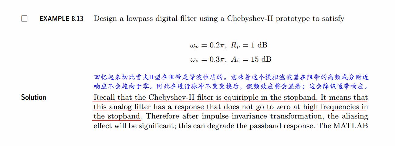
《DSP using MATLAB》示例Example 8.13

Posted 2020-09-10 沧海一粟

%% ------------------------------------------------------------------------
%%            Output Info about this m-file
fprintf(\'\\n***********************************************************\\n\');
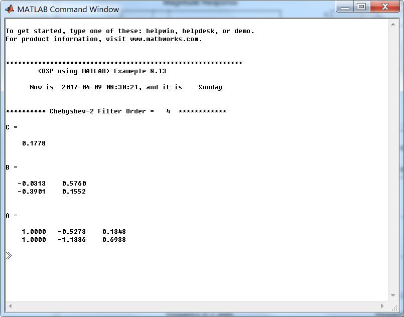
fprintf(\'        <DSP using MATLAB> Exameple 8.13 \\n\\n\');

time_stamp = datestr(now, 31);
[wkd1, wkd2] = weekday(today, \'long\');
fprintf(\'      Now is %20s, and it is %8s  \\n\\n\', time_stamp, wkd2);
%% ------------------------------------------------------------------------

% Digital Filter Specifications:
wp = 0.2*pi;                 % digital passband freq in rad
ws = 0.3*pi;                 % digital stopband freq in rad
Rp = 1;                      % passband ripple in dB
As = 15;                     % stopband attenuation in dB

% Analog prototype specifications: Inverse Mapping for frequencies
T = 1;                       % set T = 1
OmegaP = wp/T;               % prototype passband freq
OmegaS = ws/T;               % prototype stopband freq

% Analog Chebyshev-2 Prototype Filter Calculation:
[cs, ds] = afd_chb2(OmegaP, OmegaS, Rp, As);

% Impulse Invariance Transformation:
[b, a] = imp_invr(cs, ds, T); [C, B, A] = dir2par(b, a)

% Calculation of Frequency Response:
[db, mag, pha, grd, ww] = freqz_m(b, a);


%% -----------------------------------------------------------------
%%                             Plot
%% -----------------------------------------------------------------  

figure(\'NumberTitle\', \'off\', \'Name\', \'Exameple 8.13\')
set(gcf,\'Color\',\'white\'); 
M = 1;                          % Omega max

subplot(2,2,1); plot(ww/pi, mag); axis([0, M, 0, 1.2]); grid on;
xlabel(\' frequency in \\pi units\'); ylabel(\'|H|\'); title(\'Magnitude Response\');
set(gca, \'XTickMode\', \'manual\', \'XTick\', [0, 0.2, 0.3, M]);
set(gca, \'YTickMode\', \'manual\', \'YTick\', [0, 0.1778, 0.8913, 1]);

subplot(2,2,2); plot(ww/pi, pha/pi); axis([0, M, -1.1, 1.1]); grid on;
xlabel(\'frequency in \\pi nuits\'); ylabel(\'radians in \\pi units\'); title(\'Phase Response\');
set(gca, \'XTickMode\', \'manual\', \'XTick\', [0, 0.2, 0.3, M]);
set(gca, \'YTickMode\', \'manual\', \'YTick\', [-1:1:1]);

subplot(2,2,3); plot(ww/pi, db); axis([0, M, -30, 10]); grid on;
xlabel(\'frequency in \\pi units\'); ylabel(\'Decibels\'); title(\'Magnitude in dB \');
set(gca, \'XTickMode\', \'manual\', \'XTick\', [0, 0.2, 0.3, M]);
set(gca, \'YTickMode\', \'manual\', \'YTick\', [-30, -15, -1, 0]);


subplot(2,2,4); plot(ww/pi, grd); axis([0, M, 0, 15]); grid on;
xlabel(\'frequency in \\pi units\'); ylabel(\'Samples\'); title(\'Group Delay\');
set(gca, \'XTickMode\', \'manual\', \'XTick\', [0, 0.2, 0.3, M]);
set(gca, \'YTickMode\', \'manual\', \'YTick\', [0:5:15]);

　　运行结果：

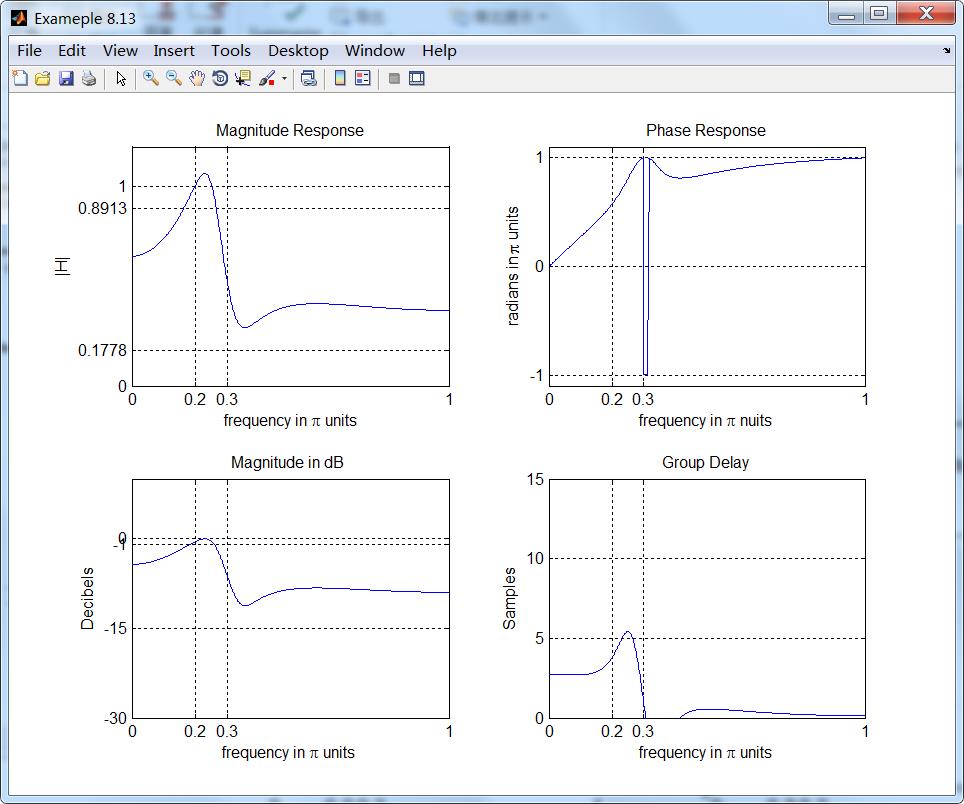
              从图中看出，通带和阻带响应都有所降级，因此脉冲不变设计方法不能够得到所需要的数字滤波器。