卷积神经网络用于视觉识别Convolutional Neural Networks for Visual Recognition

Posted 2020-06-17

Table of Contents:

• Architecture Overview
• ConvNet Layers
  • Convolutional Layer
  • Pooling Layer
  • Normalization Layer
  • Fully-Connected Layer
  • Converting Fully-Connected Layers to Convolutional Layers
• ConvNet Architectures
  • Layer Patterns
  • Layer Sizing Patterns
  • Case Studies (LeNet / AlexNet / ZFNet / GoogLeNet / VGGNet)
  • Computational Considerations
• Additional References

Convolutional Neural Networks (CNNs / ConvNets)

Convolutional Neural Networks are very similar to ordinary Neural Networks from the previous chapter: They are made up of neurons that have learnable weights and biases. Each neuron receives some inputs, performs a dot product and optionally follows it with a non-linearity. The whole network still express a single differentiable score function: From the raw image pixels on one end to class scores at the other. And they still have a loss function (e.g. SVM/Softmax) on the last (fully-connected) layer and all the tips/tricks we developed for learning regular Neural Networks still apply.

So what does change? ConvNet architectures make the explicit assumption that the inputs are images, which allows us to encode certain properties into the architecture. These then make the forward function more efficient to implement and vastly reduces the amount of parameters in the network.

Architecture Overview

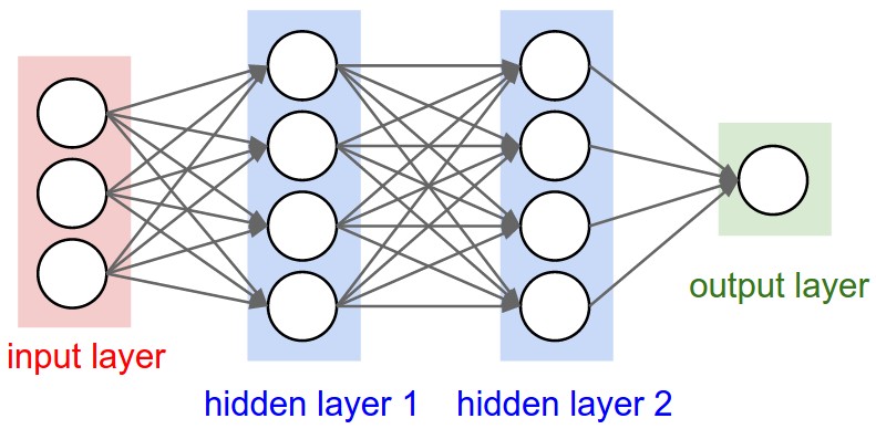
Recall: Regular Neural Nets. As we saw in the previous chapter, Neural Networks receive an input (a single vector), and transform it through a series of hidden layers. Each hidden layer is made up of a set of neurons, where each neuron is fully connected to all neurons in the previous layer, and where neurons in a single layer function completely independently and do not share any connections. The last fully-connected layer is called the "output layer" and in classification settings it represents the class scores.

Regular Neural Nets don‘t scale well to full images. In CIFAR-10, images are only of size 32x32x3 (32 wide, 32 high, 3 color channels), so a single fully-connected neuron in a first hidden layer of a regular Neural Network would have 32*32*3 = 3072 weights. This amount still seems manageable, but clearly this fully-connected structure does not scale to larger images. For example, an image of more respectible size, e.g. 200x200x3, would lead to neurons that have 200*200*3 = 120,000 weights. Moreover, we would almost certainly want to have several such neurons, so the parameters would add up quickly! Clearly, this full connectivity is wasteful and the huge number of parameters would quickly lead to overfitting.

3D volumes of neurons. Convolutional Neural Networks take advantage of the fact that the input consists of images and they constrain the architecture in a more sensible way. In particular, unlike a regular Neural Network, the layers of a ConvNet have neurons arranged in 3 dimensions: width, height, depth. (Note that the word depth here refers to the third dimension of an activation volume, not to the depth of a full Neural Network, which can refer to the total number of layers in a network.) For example, the input images in CIFAR-10 are an input volume of activations, and the volume has dimensions 32x32x3 (width, height, depth respectively). As we will soon see, the neurons in a layer will only be connected to a small region of the layer before it, instead of all of the neurons in a fully-connected manner. Moreover, the final output layer would for CIFAR-10 have dimensions 1x1x10, because by the end of the ConvNet architecture we will reduce the full image into a single vector of class scores, arranged along the depth dimension. Here is a visualization:

 

Left: A regular 3-layer Neural Network. Right: A ConvNet arranges its neurons in three dimensions (width, height, depth), as visualized in one of the layers. Every layer of a ConvNet transforms the 3D input volume to a 3D output volume of neuron activations. In this example, the red input layer holds the image, so its width and height would be the dimensions of the image, and the depth would be 3 (Red, Green, Blue channels).

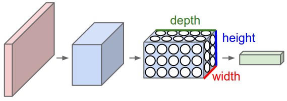
A ConvNet is made up of Layers. Every Layer has a simple API: It transforms an input 3D volume to an output 3D volume with some differentiable function that may or may not have parameters.

Layers used to build ConvNets

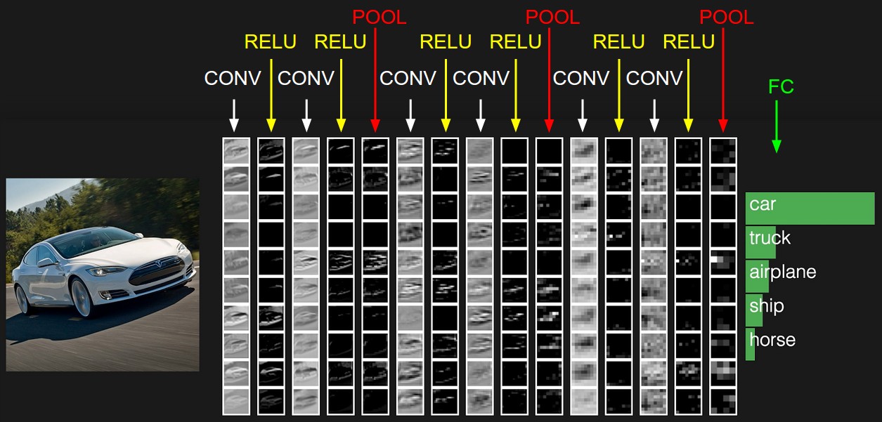
As we described above, every layer of a ConvNet transforms one volume of activations to another through a differentiable function. We use three main types of layers to build ConvNet architectures: Convolutional Layer,Pooling Layer, and Fully-Connected Layer (exactly as seen in regular Neural Networks). We will stack these layers to form a full ConvNet architecture.

Example Architecture: Overview. We will go into more details below, but a simple ConvNet for CIFAR-10 classification could have the architecture [INPUT - CONV - RELU - POOL - FC]. In more detail:

• INPUT [32x32x3] will hold the raw pixel values of the image, in this case an image of width 32, height 32, and with three color channels R,G,B.
• CONV layer will compute the output of neurons that are connected to local regions in the input, each computing a dot product between their weights and the region they are connected to in the input volume. This may result in volume such as [32x32x12].
• RELU layer will apply an elementwise activation function, such as the max(0,x)max(0,x) thresholding at zero. This leaves the size of the volume unchanged ([32x32x12]).
• POOL layer will perform a downsampling operation along the spatial dimensions (width, height), resulting in volume such as [16x16x12].
• FC (i.e. fully-connected) layer will compute the class scores, resulting in volume of size [1x1x10], where each of the 10 numbers correspond to a class score, such as among the 10 categories of CIFAR-10. As with ordinary Neural Networks and as the name implies, each neuron in this layer will be connected to all the numbers in the previous volume.

In this way, ConvNets transform the original image layer by layer from the original pixel values to the final class scores. Note that some layers contain parameters and other don‘t. In particular, the CONV/FC layers perform transformations that are a function of not only the activations in the input volume, but also of the parameters (the weights and biases of the neurons). On the other hand, the RELU/POOL layers will implement a fixed function. The parameters in the CONV/FC layers will be trained with gradient descent so that the class scores that the ConvNet computes are consistent with the labels in the training set for each image.

In summary:

• A ConvNet architecture is a list of Layers that transform the image volume into an output volume (e.g. holding the class scores)
• There are a few distinct types of Layers (e.g. CONV/FC/RELU/POOL are by far the most popular)
• Each Layer accepts an input 3D volume and transforms it to an output 3D volume through a differentiable function
• Each Layer may or may not have parameters (e.g. CONV/FC do, RELU/POOL don‘t)
• Each Layer may or may not have additional hyperparameters (e.g. CONV/FC/POOL do, RELU doesn‘t)

The activations of an example ConvNet architecture. The initial volume stores the raw image pixels and the last volume stores the class scores. Each volume of activations along the processing path is shown as a column. Since it‘s difficult to visualize 3D volumes, we lay out each volume‘s slices in rows. The last layer volume holds the scores for each class, but here we only visualize the sorted top 5 scores, and print the labels of each one. The full web-based demo is shown in the header of our website. The architecture shown here is a tiny VGG Net, which we will discuss later.

We now describe the individual layers and the details of their hyperparameters and their connectivities.

Convolutional Layer

The Conv layer is the core building block of a Convolutional Network, and its output volume can be interpreted as holding neurons arranged in a 3D volume. We now discuss the details of the neuron connectivities, their arrangement in space, and their parameter sharing scheme.

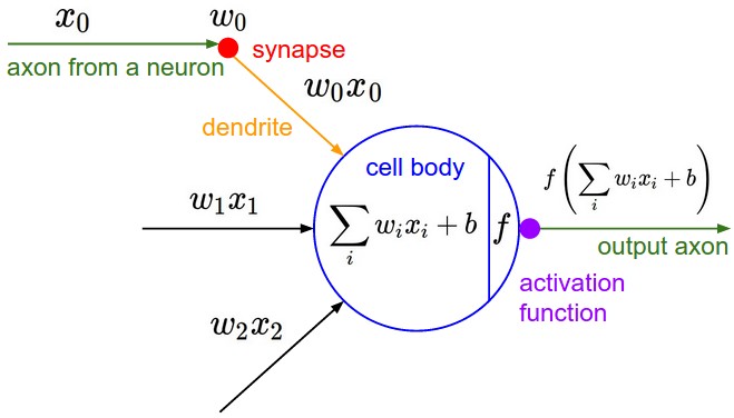
Overview and Intuition. The CONV layer‘s parameters consist of a set of learnable filters. Every filter is small spatially (along width and height), but extends through the full depth of the input volume. During the forward pass, we slide (more precisely, convolve) each filter across the width and height of the input volume, producing a 2-dimensional activation map of that filter. As we slide the filter, across the input, we are computing the dot product between the entries of the filter and the input. Intuitively, the network will learn filters that activate when they see some specific type of feature at some spatial position in the input. Stacking these activation maps for all filters along the depth dimension forms the full output volume. Every entry in the output volume can thus also be interpreted as an output of a neuron that looks at only a small region in the input and shares parameters with neurons in the same activation map (since these numbers all result from applying the same filter). We now dive into the details of this process.

Local Connectivity. When dealing with high-dimensional inputs such as images, as we saw above it is impractical to connect neurons to all neurons in the previous volume. Instead, we will connect each neuron to only a local region of the input volume. The spatial extent of this connectivity is a hyperparameter called the receptive field of the neuron. The extent of the connectivity along the depth axis is always equal to the depth of the input volume. It is important to note this asymmetry in how we treat the spatial dimensions (width and height) and the depth dimension: The connections are local in space (along width and height), but always full along the entire depth of the input volume.

Example 1. For example, suppose that the input volume has size [32x32x3], (e.g. an RGB CIFAR-10 image). If the receptive field is of size 5x5, then each neuron in the Conv Layer will have weights to a [5x5x3] region in the input volume, for a total of 5*5*3 = 75 weights. Notice that the extent of the connectivity along the depth axis must be 3, since this is the depth of the input volume.

Example 2. Suppose an input volume had size [16x16x20]. Then using an example receptive field size of 3x3, every neuron in the Conv Layer would now have a total of 3*3*20 = 180 connections to the input volume. Notice that, again, the connectivity is local in space (e.g. 3x3), but full along the input depth (20).

 

Left: An example input volume in red (e.g. a 32x32x3 CIFAR-10 image), and an example volume of neurons in the first Convolutional layer. Each neuron in the convolutional layer is connected only to a local region in the input volume spatially, but to the full depth (i.e. all color channels). Note, there are multiple neurons (5 in this example) along the depth, all looking at the same region in the input - see discussion of depth columns in text below. Right: The neurons from the Neural Network chapter remain unchanged: They still compute a dot product of their weights with the input followed by a non-linearity, but their connectivity is now restricted to be local spatially.

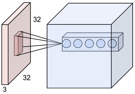
Spatial arrangement. We have explained the connectivity of each neuron in the Conv Layer to the input volume, but we haven‘t yet discussed how many neurons there are in the output volume or how they are arranged. Three hyperparameters control the size of the output volume: the depth, stride and zero-padding. We discuss these next:

1. First, the depth of the output volume is a hyperparameter that we can pick; It controls the number of neurons in the Conv layer that connect to the same region of the input volume. This is analogous to a regular Neural Network, where we had multiple neurons in a hidden layer all looking at the exact same input. As we will see, all of these neurons will learn to activate for different features in the input. For example, if the first Convolutional Layer takes as input the raw image, then different neurons along the depth dimension may activate in presence of various oriented edged, or blobs of color. We will refer to a set of neurons that are all looking at the same region of the input as a depth column.
2. Second, we must specify the stride with which we allocate depth columns around the spatial dimensions (width and height). When the stride is 1, then we will allocate a new depth column of neurons to spatial positions only 1 spatial unit apart. This will lead to heavily overlapping receptive fields between the columns, and also to large output volumes. Conversely, if we use higher strides then the receptive fields will overlap less and the resulting output volume will have smaller dimensions spatially.
3. As we will soon see, sometimes it will be convenient to pad the input with zeros spatially on the border of the input volume. The size of this zero-padding is a hyperparameter. The nice feature of zero padding is that it will allow us to control the spatial size of the output volumes. In particular, we will sometimes want to exactly preserve the spatial size of the input volume.

We can compute the spatial size of the output volume as a function of the input volume size (WW), the receptive field size of the Conv Layer neurons (FF), the stride with which they are applied (SS), and the amount of zero padding used (PP) on the border. You can convince yourself that the correct formula for calculating how many neurons "fit" is given by (W−F+2P)/S+1(W−F+2P)/S+1. If this number is not an integer, then the strides are set incorrectly and the neurons cannot be tiled so that they "fit" across the input volume neatly, in a symmetric way. An example might help to get intuitions for this formula:

Illustration of spatial arrangement. In this example there is only one spatial dimension (x-axis), one neuron with a receptive field size of F = 3, the input size is W = 5, and there is zero padding of P = 1. Left: The neuron strided across the input in stride of S = 1, giving output of size (5 - 3 + 2)/1+1 = 5. Right: The neuron uses stride of S = 2, giving output of size (5 - 3 + 2)/2+1 = 3. Notice that stride S = 3 could not be used since it wouldn‘t fit neatly across the volume. In terms of the equation, this can be determined since (5 - 3 + 2) = 4 is not divisible by 3. 
The neuron weights are in this example [1,0,-1] (shown on very right), and its bias is zero. These weights are shared across all yellow neurons (see parameter sharing below).

Use of zero-padding. In the example above on left, note that the input dimension was 5 and the output dimension was equal: also 5. This worked out so because our receptive fields were 3 and we used zero padding of 1. If there was no zero-padding used, then the output volume would have had spatial dimension of only 3, because that it is how many neurons would have "fit" across the original input. In general, setting zero padding to be P=(F−1)/2P=(F−1)/2when the stride is S=1S=1 ensures that the input volume and output volume will have the same size spatially. It is very common to use zero-padding in this way and we will discuss the full reasons when we talk more about ConvNet architectures.

Constraints on strides. Note that the spatial arrangement hyperparameters have mutual constraints. For example, when the input has size W=10W=10, no zero-padding is used P=0P=0, and the filter size is F=3F=3, then it would be impossible to use stride S=2S=2, since (W−F+2P)/S+1=(10−3+0)/2+1=4.5(W−F+2P)/S+1=(10−3+0)/2+1=4.5, i.e. not an integer, indicating that the neurons don‘t "fit" neatly and symmetrically across the input. Therefore, this setting of the hyperparameters is considered to be invalid, and a ConvNet library would likely throw an exception. As we will see in the ConvNet architectures section, sizing the ConvNets appropriately so that all the dimensions "work out" can be a real headache, which the use of zero-padding and some design guidelines will significantly alleviate.

Real-world example. The Krizhevsky et al. architecture that won the ImageNet challenge in 2012 accepted images of size [227x227x3]. On the first Convolutional Layer, it used neurons with receptive field size F=11F=11, stride S=4S=4and no zero padding P=0P=0. Since (227 - 11)/4 + 1 = 55, and since the Conv layer had a depth of K=96K=96, the Conv layer output volume had size [55x55x96]. Each of the 55*55*96 neurons in this volume was connected to a region of size [11x11x3] in the input volume. Moreover, all 96 neurons in each depth column are connected to the same [11x11x3] region of the input, but of course with different weights.

Parameter Sharing. Parameter sharing scheme is used in Convolutional Layers to control the number of parameters. Using the real-world example above, we see that there are 55*55*96 = 290,400 neurons in the first Conv Layer, and each has 11*11*3 = 363 weights and 1 bias. Together, this adds up to 290400 * 364 = 105,705,600 parameters on the first layer of the ConvNet alone. Clearly, this number is very high.

It turns out that we can dramatically reduce the number of parameters by making one reasonable assumption: That if one patch feature is useful to compute at some spatial position (x,y), then it should also be useful to compute at a different position (x2,y2). In other words, denoting a single 2-dimensional slice of depth as a depth slice (e.g. a volume of size [55x55x96] has 96 depth slices, each of size [55x55]), we are going to constrain the neurons in each depth slice to use the same weights and bias. With this parameter sharing scheme, the first Conv Layer in our example would now have only 96 unique set of weights (one for each depth slice), for a total of 96*11*11*3 = 34,848 unique weights, or 34,944 parameters (+96 biases). Alternatively, all 55*55 neurons in each depth slice will now be using the same parameters. In practice during backpropagation, every neuron in the volume will compute the gradient for its weights, but these gradients will be added up across each depth slice and only update a single set of weights per slice.

Notice that if all neurons in a single depth slice are using the same weight vector, then the forward pass of the CONV layer can in each depth slice be computed as a convolution of the neuron‘s weights with the input volume (Hence the name: Convolutional Layer). Therefore, it is common to refer to the sets of weights as a filter (or a kernel), which is convolved with the input. The result of this convolution is an activation map (e.g. of size [55x55]), and the set of activation maps for each different filter are stacked together along the depth dimension to produce the output volume (e.g. [55x55x96]).

Example filters learned by Krizhevsky et al. Each of the 96 filters shown here is of size [11x11x3], and each one is shared by the 55*55 neurons in one depth slice. Notice that the parameter sharing assumption is relatively reasonable: If detecting a horizontal edge is important at some location in the image, it should intuitively be useful at some other location as well due to the translationally-invariant structure of images. There is therefore no need to relearn to detect a horizontal edge at every one of the 55*55 distinct locations in the Conv layer output volume.

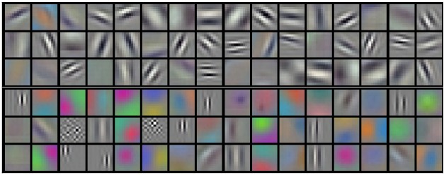
Note that sometimes the parameter sharing assumption may not make sense. This is especially the case when the input images to a ConvNet have some specific centered structure, where we should expect, for example, that completely different features should be learned on one side of the image than another. One practical example is when the input are faces that have been centered in the image. You might expect that different eye-specific or hair-specific features could (and should) be learned in different spatial locations. In that case it is common to relax the parameter sharing scheme, and instead simply call the layer a Locally-Connected Layer.

Numpy examples. To make the discussion above more concrete, lets express the same ideas but in code and with a specific example. Suppose that the input volume is a numpy array X. Then:

• A depth column at position (x,y) would be the activations X[x,y,:].
• A depth slice, or equivalently an activation map at depth d would be the activations X[:,:,d].

Conv Layer Example. Suppose that the input volume X has shape X.shape: (11,11,4). Suppose further that we use no zero padding (P=0P=0), that the filter size is F=5F=5, and that the stride is S=2S=2. The output volume would therefore have spatial size (11-5)/2+1 = 4, giving a volume with width and height of 4. The activation map in the output volume (call it V), would then look as follows (only some of the elements are computed in this example):

• V[0,0,0] = np.sum(X[:5,:5,:] * W0) + b0
• V[1,0,0] = np.sum(X[2:7,:5,:] * W0) + b0
• V[2,0,0] = np.sum(X[4:9,:5,:] * W0) + b0
• V[3,0,0] = np.sum(X[6:11,:5,:] * W0) + b0

Remember that in numpy, the operation * above denotes elementwise multiplication between the arrays. Notice also that the weight vector W0 is the weight vector of that neuron and b0 is the bias. Here, W0 is assumed to be of shape W0.shape: (5,5,4), since the filter size is 5 and the depth of the input volume is 4. Notice that at each point, we are computing the dot product as seen before in ordinary neural networks. Also, we see that we are using the same weight and bias (due to parameter sharing), and where the dimensions along the width are increasing in steps of 2 (i.e. the stride). To construct a second activation map in the output volume, we would have:

• V[0,0,1] = np.sum(X[:5,:5,:] * W1) + b1
• V[1,0,1] = np.sum(X[2:7,:5,:] * W1) + b1
• V[2,0,1] = np.sum(X[4:9,:5,:] * W1) + b1
• V[3,0,1] = np.sum(X[6:11,:5,:] * W1) + b1
• V[0,1,1] = np.sum(X[:5,2:7,:] * W1) + b1 (example of going along y)
• V[2,3,1] = np.sum(X[4:9,6:11,:] * W1) + b1 (or along both)

where we see that we are indexing into the second depth dimension in V (at index 1) because we are computing the second activation map, and that a different set of parameters (W1) is now used. In the example above, we are for brevity leaving out some of the other operatations the Conv Layer would perform to fill the other parts of the output array V. Additionally, recall that these activation maps are often followed elementwise through an activation function such as ReLU, but this is not shown here.

Summary. To summarize, the Conv Layer:

• Accepts a volume of size W1×H1×D1W1×H1×D1
• Requires four hyperparameters:
  • Number of filters KK,
  • their spatial extent FF,
  • the stride SS,
  • the amount of zero padding PP.
• Produces a volume of size W2×H2×D2W2×H2×D2 where:
  • W2=(W1−F+2P)/S+1W2=(W1−F+2P)/S+1
  • H2=(H1−F+2P)/S+1H2=(H1−F+2P)/S+1 (i.e. width and height are computed equally by symmetry)
  • D2=KD2=K
• With parameter sharing, it introduces F⋅F⋅D1F⋅F⋅D1 weights per filter, for a total of (F⋅F⋅D1)⋅K(F⋅F⋅D1)⋅K weights and KK biases.
• In the output volume, the dd-th depth slice (of size W2×H2W2×H2) is the result of performing a valid convolution of the dd-th filter over the input volume with a stride of SS, and then offset by dd-th bias.

A common setting of the hyperparameters is F=3,S=1,P=1F=3,S=1,P=1. However, there are common conventions and rules of thumb that motivate these hyperparameters. See the ConvNet architectures section below.

Convolution Demo. Below is a running demo of a CONV layer. Since 3D volumes are hard to visualize, all the volumes (the input volume (in blue), the weight volumes (in red), the output volume (in green)) are visualized with each depth slice stacked in rows. The input volume is of size W1=5,H1=5,D1=3W1=5,H1=5,D1=3, and the CONV layer parameters are K=2,F=3,S=2,P=1K=2,F=3,S=2,P=1. That is, we have two filters of size 3×33×3, and they are applied with a stride of 2. Therefore, the output volume size has spatial size (5 - 3 + 2)/2 + 1 = 3. Moreover, notice that a padding of