understanding backpropagation

Posted 2020-08-20 cslxiao

几个有助于加深对反向传播算法直观理解的网页，包括普通前向神经网络，卷积神经网络以及利用BP对一般性函数求导（UFLDL）

 

A Visual Explanation of the Back Propagation Algorithm for Neural Networks

By Sebastian Raschka, Michigan State University.

Let‘s assume we are really into mountain climbing, and to add a little extra challenge, we cover eyes this time so that we can‘t see where we are and when we accomplished our "objective," that is, reaching the top of the mountain.

Since we can‘t see the path upfront, we let our intuition guide us: assuming that the mountain top is the "highest" point of the mountain, we think that the steepest path leads us to the top most efficiently.

We approach this challenge by iteratively "feeling" around you and taking a step into the direction of the steepest ascent -- let‘s call it "gradient ascent." But what do we do if we reach a point where we can‘t ascent any further? I.e., each direction leads downwards? At this point, we may have already reached the mountain‘s top, but we could just have reached a smaller plateau ... we don‘t know. Essentially, this is just an analogy of gradient ascent optimization (basically the counterpart of minimizing a cost function via gradient descent). However, this is not specific to backpropagation but just one way to minimize a convex cost function (if there is only a global minima) or non-convex cost function (which has local minima like the "plateaus" that let us think we reached the mountain‘s top). Using a little visual aid, we could picture a non-convex cost function with only one parameter (where the blue ball is our current location) as follows:

Now, backpropagation is just back-propagating the cost over multiple "levels" (or layers). E.g., if we have a multi-layer perceptron, we can picture forward propagation (passing the input signal through a network while multiplying it by the respective weights to compute an output) as follows:

And in backpropagation, we "simply" backpropagate the error (the "cost" that we compute by comparing the calculated output and the known, correct target output, which we then use to update the model parameters):

It may be some time ago since pre-calc, but it‘s essentially all based on the simple chain-rule that we use for nested functions

 

Instead of doing this "manually" we can use computational tools (called "automatic differentiation"), and backpropagation is basically the "reverse" mode of this auto-differentiation. Why reverse and not forward? Because it is computationally cheaper! If we‘d do it forward-wise, we‘d successively multiply large matrices for each layer until we multiply a large matrix by a vector in the output layer. However, if we start backwards, that is, we start by multiplying a matrix by a vector, we get another vector, and so forth. So, I‘d say the beauty in backpropagation is that we are doing more efficient matrix-vector multiplications instead of matrix-matrix multiplications.

 

 

 

 

 

 

 

 

 

 

 

Deriving gradients using the backpropagation idea

From UFLDL tutorial

 

Introduction

In the section on the backpropagation algorithm, you were briefly introduced to backpropagation as a means of deriving gradients for learning in the sparse autoencoder. It turns out that together with matrix calculus, this provides a powerful method and intuition for deriving gradients for more complex matrix functions (functions from matrices to the reals, or symbolically, from ).

First, recall the backpropagation idea, which we present in a modified form appropriate for our purposes below:

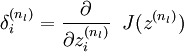
1. For each output unit i in layer n_l (the final layer), set

   

   where J(z) is our "objective function" (explained below).
2. For 

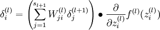
   For each node i in layer l, set

   

3. Compute the desired partial derivatives,

   

Quick notation recap:

• l is the number of layers in the neural network
• n_l is the number of neurons in the lth layer
•  is the weight from the ith unit in the lth layer to the jth unit in the (l + 1)th layer
•  is the input to the ith unit in the lth layer
•  is the activation of the ith unit in the lth layer
•  is the Hadamard or element-wise product, which for  matrices A and B yields the  matrix  such that 
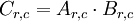
• f^(l) is the activation function for units in the lth layer

Let‘s say we have a function F that takes a matrix X and yields a real number. We would like to use the backpropagation idea to compute the gradient with respect to X of F, that is . The general idea is to see the function F as a multi-layer neural network, and to derive the gradients using the backpropagation idea.

To do this, we will set our "objective function" to be the function J(z) that when applied to the outputs of the neurons in the last layer yields the value F(X). For the intermediate layers, we will also choose our activation functions f^(l) to this end.

Using this method, we can easily compute derivatives with respect to the inputs X, as well as derivatives with respect to any of the weights in the network, as we shall see later.

Examples

To illustrate the use of the backpropagation idea to compute derivatives with respect to the inputs, we will use two functions from the section onsparse coding, in examples 1 and 2. In example 3, we use a function from independent component analysis to illustrate the use of this idea to compute derivates with respect to weights, and in this specific case, what to do in the case of tied or repeated weights.

Example 1: Objective for weight matrix in sparse coding

Recall for sparse coding, the objective function for the weight matrix A, given the feature matrix s:

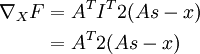
We would like to find the gradient of F with respect to A, or in symbols, . Since the objective function is a sum of two terms in A, the gradient is the sum of gradients of each of the individual terms. The gradient of the second term is trivial, so we will consider the gradient of the first term instead.

The first term, , can be seen as an instantiation of neural network taking s as an input, and proceeding in four steps, as described and illustrated in the paragraph and diagram below:

1. Apply A as the weights from the first layer to the second layer.
2. Subtract x from the activation of the second layer, which uses the identity activation function.
3. Pass this unchanged to the third layer, via identity weights. Use the square function as the activation function for the third layer.
4. Sum all the activations of the third layer.

The weights and activation functions of this network are as follows:

Layer	Weight	Activation function f
1	A	f(zi) = zi (identity)
2	I (identity)	f(zi) = zi ? xi
3	N/A

To have J(z⁽³⁾) = F(x), we can set .

Once we see F as a neural network, the gradient  becomes easy to compute - applying backpropagation yields:

Layer	Derivative of activation function f‘	Delta	Input z to this layer
3	f‘(zi) = 2zi	f‘(zi) = 2zi	As ? x
2	f‘(zi) = 1		As
1	f‘(zi) = 1		s

Hence,

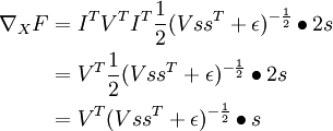
Example 2: Smoothed topographic L1 sparsity penalty in sparse coding

Recall the smoothed topographic L1 sparsity penalty on s in sparse coding:

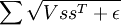
where V is the grouping matrix, s is the feature matrix and ε is a constant.

We would like to find 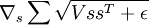. As above, let‘s see this term as an instantiation of a neural network:

The weights and activation functions of this network are as follows:

Layer	Weight	Activation function f
1	I
2	V	f(zi) = zi
3	I	f(zi) = zi + ε
4	N/A

To have J(z⁽⁴⁾) = F(x), we can set .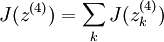

Once we see F as a neural network, the gradient  becomes easy to compute - applying backpropagation yields:

Layer	Derivative of activation function f‘	Delta	Input z to this layer
4		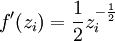	(VssT + ε)
3	f‘(zi) = 1		VssT
2	f‘(zi) = 1		ssT
1	f‘(zi) = 2zi		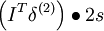s

Hence,

Example 3: ICA reconstruction cost

Recall the independent component analysis (ICA) reconstruction cost term: 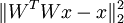 where W is the weight matrix and x is the input.

We would like to find 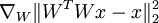 - the derivative of the term with respect to the weight matrix, rather than the input as in the earlier two examples. We will still proceed similarly though, seeing this term as an instantiation of a neural network:

The weights and activation functions of this network are as follows:

Layer	Weight	Activation function f
1	W	f(zi) = zi
2	WT	f(zi) = zi
3	I	f(zi) = zi ? xi
4	N/A

To have J(z⁽⁴⁾) = F(x), we can set .

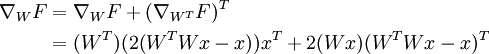
Now that we can see F as a neural network, we can try to compute the gradient . However, we now face the difficulty that W appears twice in the network. Fortunately, it turns out that if W appears multiple times in the network, the gradient with respect to W is simply the sum of gradients for each instance of W in the network (you may wish to work out a formal proof of this fact to convince yourself). With this in mind, we will proceed to work out the deltas first:

Layer	Derivative of activation function f‘	Delta	Input z to this layer
4	f‘(zi) = 2zi	f‘(zi) = 2zi	(WTWx ? x)
3	f‘(zi) = 1		WTWx
2	f‘(zi) = 1		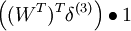Wx
1	f‘(zi) = 1		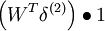x

To find the gradients with respect to W, first we find the gradients with respect to each instance of W in the network.

With respect to W^T:

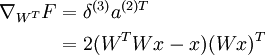
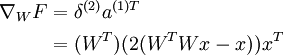
With respect to W:

Taking sums, noting that we need to transpose the gradient with respect to W^T to get the gradient with respect to W, yields the final gradient with respect to W (pardon the slight abuse of notation here):

 

 

 

 

 

 

 

 

 

 

 

Convolutional Neural Networks backpropagation: from intuition to derivation

Disclaimer: It is assumed that the reader is familiar with terms such as Multilayer Perceptron, delta errors or backpropagation. If not,  it is recommended to read for example a chapter 2 of free online book ‘Neural Networks and Deep Learning’ byMichael Nielsen.   

Convolutional Neural Networks (CNN) are now a standard way of image classification – there are publicly accessible deep learning frameworks, trained models and services. It’s more time consuming to install stuff like caffe than to perform state-of-the-art object classification or detection. We also have many methods of getting knowledge -there is a large number of deep learning courses/MOOCs, free e-books or even direct ways of accessing to the strongest Deep/Machine Learning minds such as Yoshua Bengio, Andrew NG or Yann Lecun by Quora, Facebook or G+.

Nevertheless, when I wanted to get deeper insight in CNN, I could not find a “CNN backpropagation for dummies”. Notoriously I met with statements like:  “If you understand backpropagation in standard neural networks, there should not be a problem with understanding it in CNN” or “All things are nearly the same, except matrix multiplications are replaced by convolutions”. And of course I saw tons of ready equations.

It was a little consoling, when I found out that I am not alone, for example: Hello, when computing the gradients CNN,  the weights need to be rotated, Why ? 

The answer on above question, that concerns the need of rotation on weights in gradient computing, will be a result of this long post.

We start from multilayer perceptron and counting delta errors on fingers:

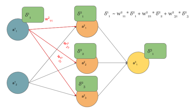
We see on above picture that  is proportional to deltas from next layer that are scaled by weights.

But how do we connect concept of MLP with Convolutional Neural Network? Let’s play with MLP:

Transforming Multilayer Perceptron to Convolutional Neural Network

If you are not sure that after connections cutting and weights sharing we get one layer Convolutional Neural Network, I hope that below picture will convince you:

Feedforward in CNN is identical with convolution operation

The idea behind this figure is to show, that such neural network configuration  is identical with a 2D convolution operation and weights are just filters (also called kernels, convolution matrices, or masks).

Now we can come back to gradient computing by counting on fingers, but from now we will be only focused on CNN. Let’s begin:

Backpropagation also results with convolution

No magic here, we have just summed in “blue layer” scaled by weights gradients from “orange” layer. Same process as in MLP’s backpropagation. However, in the standard approach we talk about dot products and here we have … yup, again convolution:

Yeah, it is a bit different convolution than in previous (forward) case. There we did so called valid convolution, while here we do a full convolution (more about nomenclaturehere). What is more, we rotate our kernel by 180 degrees. But still, we are talking about convolution!

Now, I have some good news and some bad news:

1. you see (BTW, sorry for pictures aesthetics :) ), that matrix dot products are replaced by convolution operations both in feed forward and backpropagation.
2. you know that seeing something and understanding something … yup, we are going now to get our hands dirty and prove above statement <fn> before getting next, I recommend to read, mentioned already in the disclaimer, chapter 2 of M. Nielsen book. I tried to make all quantities to be consistent with work of Michael. 

In the standard MLP, we can define an error of neuron j as:

where  is just:

and for clarity,  , where  is an activation function such as sigmoid, hyperbolic tangent or relu.

But here, we do not have MLP but CNN and matrix multiplications are replaced by convolutions as we discussed before. So instead of   we do have a :

Above equation is just a convolution operation during feedforward phase illustrated in the above picture titled ‘Feedforward in CNN is identical with convolution operation’

Now we can get to the point and answer the question Hello, when computing the gradients CNN,  the weights need to be rotated, Why ? 

We start from statement:

We know that  is in relation to  which is indirectly showed in  the above picture titled ‘Backpropagation also results with convolution’. So sums are the result of chain rule. Let’s move on:

First term is replaced by definition of error, while second has become large because we put it here expression on . However, we do not have to fear of this big monster – all components of sums equal 0, except these ones that are indexed:  and . So:

If  and  then it is obvious that  and  so we can reformulate above equation to:

 

OK, our last equation is just …

 

Where is the rotation of weights? Actually .

So the answer on question Hello, when computing the gradients CNN,  the weights need to be rotated, Why ?  is simple: the rotation of the weights just results from derivation of delta error in Convolution Neural Network.

OK, we are really close to the end. One more ingredient of backpropagation algorithm is update of weights :

So paraphrasing the backpropagation algorithm  for CNN:

1. Input x: set the corresponding activation  for the input layer.
2. Feedforward: for each l = 2,3, …,L compute  and 
3. Output error : Compute the vector 
4. Backpropagate the error: For each l=L-1,L-2,…,2 compute 
5. Output: The gradient of the cost function is given by 

The end

 

 

 

 

 

 

 

 

Why do we rotate weights when computing the gradients in a convolution layer of a convolution network?

 

Today someone asked on Google+

Hello, when computing the gradients CNN, the weights need to be rotated, Why ?

I had the same question when I was pouring through code back in the day, so I wanted to clear it up for people once and for all.

Simple answer:

This is just a efficient and clean way of writing things for:

Computing the gradient of a valid 2D convolution w.r.t. the inputs.

There is no magic here

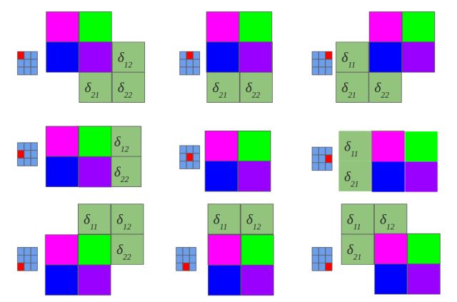
Here’s a detailed explanation with visualization!

Input  Kernel  Output 

Section 1: valid convolution (input, kernel)

Section 2: gradient w.r.t. input of valid convolution (input, kernel) = weighted contribution of each input location w.r.t. gradient of Output

Section 3: full convolution(180 degree rotated filter, output)

As you can see, the calculation for the first three elements in section 2 is the same as the first three figures in section 3.

Hope this helps!