转载 Deep learning：四(logistic regression练习)

Posted 2020-08-03 我是一个粉刷匠

前言：

本节来练习下logistic regression相关内容，参考的资料为网页：http://openclassroom.stanford.edu/MainFolder/DocumentPage.php?course=DeepLearning&doc=exercises/ex4/ex4.html。这里给出的训练样本的特征为80个学生的两门功课的分数，样本值为对应的同学是否允许被上大学，如果是允许的话则用’1’表示，否则不允许就用’0’表示，这是一个典型的二分类问题。在此问题中，给出的80个样本中正负样本各占40个。而这节采用的是logistic regression来求解，该求解后的结果其实是一个概率值，当然通过与0.5比较就可以变成一个二分类问题了。

实验基础：

在logistic regression问题中，logistic函数表达式如下：

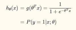
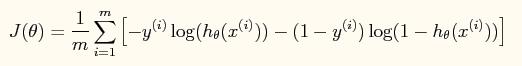
这样做的好处是可以把输出结果压缩到0~1之间。而在logistic回归问题中的损失函数与线性回归中的损失函数不同，这里定义的为：

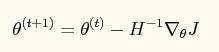
如果采用牛顿法来求解回归方程中的参数，则参数的迭代公式为：

其中一阶导函数和hessian矩阵表达式如下：

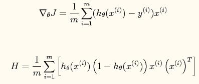
当然了，在编程的时候为了避免使用for循环，而应该直接使用这些公式的矢量表达式（具体的见程序内容）。

一些matlab函数：

find:

是找到的一个向量，其结果是find函数括号值为真时的值的下标编号。

inline:

构造一个内嵌的函数，很类似于我们在草稿纸上写的数学推导公式一样。参数一般用单引号弄起来，里面就是函数的表达式，如果有多个参数，则后面用单引号隔开一一说明。比如：g = inline(\'sin(alpha*x)\',\'x\',\'alpha\')，则该二元函数是g(x,alpha) = sin(alpha*x)。

实验结果：

训练样本的分布图以及所学习到的分类界面曲线：

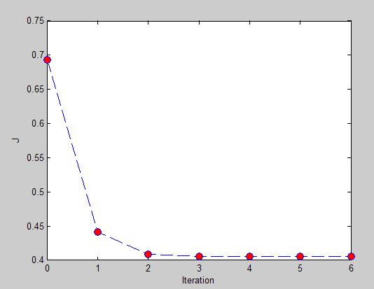
损失函数值和迭代次数之间的曲线：

最终输出的结果：

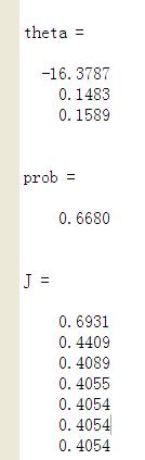
可以看出当一个小孩的第一门功课为20分，第二门功课为80分时，这个小孩不允许上大学的概率为0.6680，因此如果作为二分类的话，就说明该小孩不会被允许上大学。

实验代码（原网页提供）：

% Exercise 4 -- Logistic Regression

clear all; close all; clc

x = load(\'ex4x.dat\'); 
y = load(\'ex4y.dat\');

[m, n] = size(x);

% Add intercept term to x
x = [ones(m, 1), x]; 

% Plot the training data
% Use different markers for positives and negatives
figure
pos = find(y); neg = find(y == 0);%find是找到的一个向量，其结果是find函数括号值为真时的值的编号
plot(x(pos, 2), x(pos,3), \'+\')
hold on
plot(x(neg, 2), x(neg, 3), \'o\')
hold on
xlabel(\'Exam 1 score\')
ylabel(\'Exam 2 score\')


% Initialize fitting parameters
theta = zeros(n+1, 1);

% Define the sigmoid function
g = inline(\'1.0 ./ (1.0 + exp(-z))\'); 

% Newton\'s method
MAX_ITR = 7;
J = zeros(MAX_ITR, 1);

for i = 1:MAX_ITR
    % Calculate the hypothesis function
    z = x * theta;
    h = g(z);%转换成logistic函数
    
    % Calculate gradient and hessian.
    % The formulas below are equivalent to the summation formulas
    % given in the lecture videos.
    grad = (1/m).*x\' * (h-y);%梯度的矢量表示法
    H = (1/m).*x\' * diag(h) * diag(1-h) * x;%hessian矩阵的矢量表示法
    
    % Calculate J (for testing convergence)
    J(i) =(1/m)*sum(-y.*log(h) - (1-y).*log(1-h));%损失函数的矢量表示法
    
    theta = theta - H\\grad;%是这样子的吗？
end
% Display theta
theta

% Calculate the probability that a student with
% Score 20 on exam 1 and score 80 on exam 2 
% will not be admitted
prob = 1 - g([1, 20, 80]*theta)

%画出分界面
% Plot Newton\'s method result
% Only need 2 points to define a line, so choose two endpoints
plot_x = [min(x(:,2))-2,  max(x(:,2))+2];
% Calculate the decision boundary line，plot_y的计算公式见博客下面的评论。
plot_y = (-1./theta(3)).*(theta(2).*plot_x +theta(1));
plot(plot_x, plot_y)
legend(\'Admitted\', \'Not admitted\', \'Decision Boundary\')
hold off

% Plot J
figure
plot(0:MAX_ITR-1, J, \'o--\', \'MarkerFaceColor\', \'r\', \'MarkerSize\', 8)
xlabel(\'Iteration\'); ylabel(\'J\')
% Display J
J

参考资料：

http://openclassroom.stanford.edu/MainFolder/DocumentPage.php?course=DeepLearning&doc=exercises/ex4/ex4.html

作者：tornadomeet 出处：http://www.cnblogs.com/tornadomeet 欢迎转载或分享，但请务必声明文章出处。