Generating Sankey Diagrams from rCharts

Posted 2020-07-23 payton数据之旅

A couple of weeks or so ago, I picked up an inlink from an OCLC blog post about Visualizing Network Flows: Library Inter-lending. The post made use of Sankey diagrams to represent borrowing flows, and by implication suggested that the creation of such diagrams is not as easy as it could be…

Around the same time, @tiemlyportfolio posted a recipe for showing how to wrap custom charts so that they could be called from the amazing javascript graphics library wrapping rCharts (more about this in a forthcoming post somewhere…). rCharts Extra – d3 Horizon Conversion provides a walkthrough demonstrating how to wrap a d3.js implemented horizon chart so that it can be generated from R with what amounts to little more than a single line of code. So I idly tweeted a thought wondering how easy it would be to run through the walkthrough and try wrapping a Sankey diagram in the same way (I didn’t have time to try it myself at that moment in time.)

Within a few days, @timelyportfolio had come up with the goods – Exploring Networks with Sankey and then a further follow on post: All My Roads Lead Back to Finance–PIMCO Sankey. The code itself can be found athttps://github.com/timelyportfolio/rCharts_d3_sankey

Somehow, playtime has escaped me for the last couple of weeks, but I finally got round to trying the recipe out. The data I opted for is energy consumption data for the UK, published by DECC, detailing energy use in 2010.

As ever, we can’t just dive straight into the visualiastion – we need to do some work first to get int into shape… The data came as a spreadsheet with the following table layout:

The Sankey diagram generator requires data in three columns – source, target and value – describing what to connect to what and with what thickness line. Looking at the data, I thought it might be interesting to try to represent as flows the amount of each type of energy used by each sector relative to end use, or something along those lines (I just need something authentic to see if I can get @timelyportfolio’s recipe to work;-) So it looks as if some shaping is in order…

To tidy and reshape the data, I opted to use OpenRefine, copying and pasting the data into a new OpenRefine project:

The data is tab separated and we can ignore empty lines:

Here’s the data as loaded. You can see several problems with it: numbers that have commas in them; empty cells marked as blank or with a -; empty/unlabelled cells.

Let’s make a start by filling in the blank cells in the Sector column – Fill down:

We don’t need the overall totals because we want to look at piecewise relations (and if we do need the totals, we can recalculate them anyway):

To tidy up the numbers so they actually are numbers, we’re going to need to do some transformations:

There are several things to do: remove commas, remove – signs, and cast things as numbers:

value.replace(‘,‘,‘‘) says replace commas with an empty string (ie nothing – delete the comma).

We can then pass the result of this transformation into a following step – replace the – signs:value.replace(‘,‘,‘‘).replace(‘-‘,‘‘)

Then turn the result into a number: value.replace(‘,‘,‘‘).replace(‘-‘,‘‘).toNumber()

If there’s an error, not that we select to set the cell to a blank.

having run this transformation on one column, we can select Transform on another column and just reuse the transformation (remembering to set the cell to blank if there is an error):

To simplify the dataset further, let’s get rid of he other totals data:

Now we need to reshape the data – ideally, rather than having columns for each energy type, we want to relate the energy type to each sector/end use pair. We’re going to have to transpose the data…

So let’s do just that – wrap columns down into new rows:

We’re going to need to fill down again…

So now we have our dataset, which can be trivially exported as a CSV file:

Data cleaning and shaping phase over, we’re now ready to generate the Sankey diagram…

As ever, I’m using RStudio as my R environment. Load in the data:

To start, let’s do a little housekeeping:

#Here’s the baseline column naming for the dataset
colnames(DECC.overall.energy)=c(‘Sector’,’Enduse’,’EnergyType’,’value’)

1 2 3 4 5 6 7 8 9 10 11 12 13 14 15 16 17 18 19

#Inspired by @timelyportfolio - All My Roads Lead Back to Finance–PIMCO Sankey #http://timelyportfolio.blogspot.co.uk/2013/07/all-my-roads-lead-back-to-financepimco.html   #Now let‘s create a Sankey diagram - we need to install RCharts ##http://ramnathv.github.io/rCharts/ require(rCharts)   #Download and unzip @timelyportfolio‘s Sankey/rCharts package #Take note of where you put it! #https://github.com/timelyportfolio/rCharts_d3_sankey   sankeyPlot <- rCharts$new()   #We need to tell R where the Sankey library is. #I put it as a subdirectory to my current working directory (.) sankeyPlot$setLib(‘./rCharts_d3_sankey-gh-pages/‘)   #We also need to point to an html template page sankeyPlot$setTemplate(script = "./rCharts_d3_sankey-gh-pages/layouts/chart.html")

having got everything set up, we can cast the data into the form the Sankey template expects – with source, target and value columns identified:

1 2 3 4 5 6 7

#The plotting routines require column names to be specified as: ##source, target, value #to show what connects to what and by what thickness line   #If we want to plot from enduse to energytype we need this relabelling workingdata=DECC.overall.energy colnames(workingdata)=c(‘Sector‘,‘source‘,‘target‘,‘value‘)

Following @timelyportfolio, we configure the chart and then open it to a browser window:

1 2 3 4 5 6 7 8 9 10 11

sankeyPlot$set(   data = workingdata,   nodeWidth = 15,   nodePadding = 10,   layout = 32,   width = 750,   height = 500,   labelFormat = ".1%" )   sankeyPlot

Here’s the result:

Let’s make plotting a little easier by wrapping that routine into a function:

1 2 3 4 5 6 7 8 9 10 11 12 13 14 15 16 17 18 19 20 21 22 23 24 25 26

#To make things easier, let‘s abstract a little more... sankeyPlot=function(df){   sankeyPlot <- rCharts$new()       #--------   #See note in PPS to this post about a simplification of this part....   #We need to tell R where the Sankey library is.   #I put it as a subdirectory to my current working directory (.)   sankeyPlot$setLib(‘./rCharts_d3_sankey-gh-pages/‘)       #We also need to point to an HTML template page   sankeyPlot$setTemplate(script = "./rCharts_d3_sankey-gh-pages/layouts/chart.html")   #---------      sankeyPlot$set(     data = df,     nodeWidth = 15,     nodePadding = 10,     layout = 32,     width = 750,     height = 500,     labelFormat = ".1%"   )       sankeyPlot }

Now let’s try plotting something a little more adventurous:

1 2 3 4 5 6 7 8 9 10 11 12

#If we want to add in a further layer, showing how each Sector contributes #to the End-use energy usage, we need to additionally treat the Sector as #a source and the sum of that sector‘s energy use by End Use #Recover the colnames so we can see what‘s going on sectorEnergy=aggregate(value ~ Sector + Enduse, DECC.overall.energy, sum) colnames(sectorEnergy)=c(‘source‘,‘target‘,‘value‘)   #We can now generate a single data file combing all source and target data energyfull=subset(workingdata,select=c(‘source‘,‘target‘,‘value‘)) energyfull=rbind(energyfull,sectorEnergy)   sankeyPlot(energyfull)

And the result?

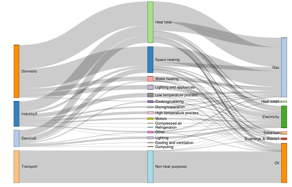
Notice that the bindings are a little bit fractured – for example, the Heat block has several contributions from the Gas block. This also suggests that a Sankey diagram, at least as configured above, may not be the most appropriate way of representing the data in this case. Sankey diagrams are intended to represent flows, which means that there is a notion of some quantity flowing between elements, and further that that quantity is conserved as it passes through each element (sum of inputs equals sum of outputs).

A more natural story might be to show Energy type flowing to end use and then out to Sector, at least if we want to see how energy is tending to be used for what purpose, and then how end use is split by Sector. However, such a diagram would not tell us, for example, that Sector X was dominated in its use of energy source A for end use P, compared to Sector Y mainly using energy source B for the same end use P.

One approach we might take to tidying up the chart to make it more readable (for some definition of readable!), though at the risk of making it even more misleading, is to do a little bit more aggregation of the data, and then bind appropriate blocks together. Here are a few more examples of simple aggregations:

We can also explore other relationships and trivially generate corresponding Sankey diagram views over them:

1 2 3 4 5 6 7 8 9 10 11 12 13

#How much of each energy type does each sector use enduseBySector=aggregate(value ~ Sector + Enduse, DECC.overall.energy, sum) colnames(enduseBySector)=c(‘source‘,‘target‘,‘value‘) sankeyPlot(enduseBySector)   colnames(enduseBySector)=c(‘target‘,‘source‘,‘value‘) sankeyPlot(enduseBySector)   #How much of each energy type is associated with each enduse energyByEnduse=aggregate(value ~ EnergyType + Enduse, DECC.overall.energy, sum) colnames(energyByEnduse)=c(‘source‘,‘target‘,‘value‘)   sankeyPlot(energyByEnduse)

So there we have it – quick and easy Sankey diagrams from R using rCharts and magic recipe from @timelyportfolio:-)

PS the following routine makes it easier to grab data into the appropriately named format

1 2 3 4 5 6 7 8 9 10 11 12

#This routine makes it easier to get the data for plotting as a Sankey diagram #Select the source, target and value column names explicitly to generate a dataframe containing #just those columns, appropriately named. sankeyData=function(df,colsource=‘source‘,coltarget=‘target‘,colvalue=‘value‘){   sankey.df=subset(df,select=c(colsource,coltarget,colvalue))   colnames(sankey.df)=c(‘source‘,‘target‘,‘value‘)   sankey.df }   #For example: data.sdf=sankeyData(DECC.overall.energy,‘Sector‘,‘EnergyType‘,‘value‘) data.sdf

The code automatically selects the appropriate columns and renames them as required.

PPS it seems that a recent update(?) to the rCharts library by @ramnath_vaidya now makes things even easier and removes the need to download and locally host @timelyportfolio’s code:

1 2 3 4 5

#We can remove the local dependency and replace the following... #sankeyPlot$setLib(‘./rCharts_d3_sankey-gh-pages/‘) #sankeyPlot$setTemplate(script = "./rCharts_d3_sankey-gh-pages/layouts/chart.html") ##with this simplification sankeyPlot$setLib(‘http://timelyportfolio.github.io/rCharts_d3_sankey‘)