求解一道matlab curve fitting的题目，求大神速解。

Posted 2023-04-30

求解一道matlab curve fitting的题目变了X与Y之间的关系是Y=a*X-a*x^2采集到的数据是 X = [0.028 0.049 0.209 0.324 0.421 0.536 0.613 0.716 0.813 0.897 0.922]; Y = [0.055 0.069 0.569 1.234 1.324 1.567 1.421 1.650 1.581 0.770 0.610];用MATLAB求a值，并且画出X和Y 的图像

参考技术A

cftool拟合工具箱

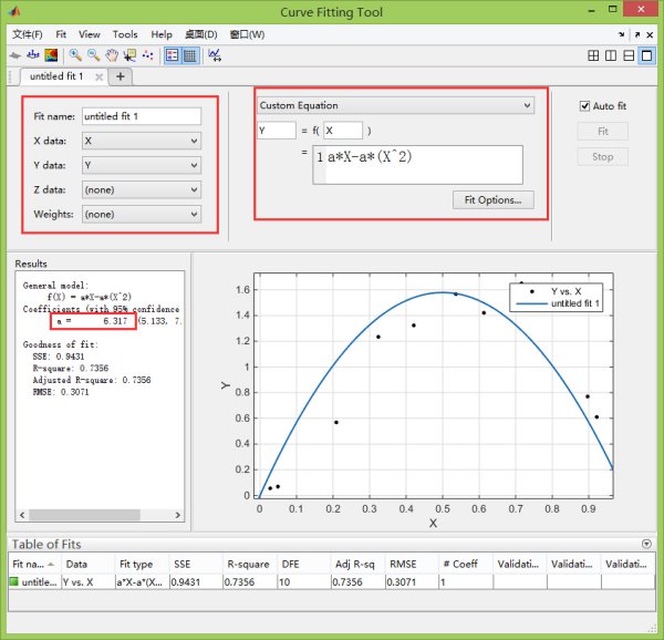
命令行窗口里输入X = [0.028 0.049 0.209 0.324 0.421 0.536 0.613 0.716 0.813 0.897 0.922]; Y = [0.055 0.069 0.569 1.234 1.324 1.567 1.421 1.650 1.581 0.770 0.610];

左上角的参数里进行设置：X data选择变量X，Y data选择变量Y；

拟合类型选择Custom Equation，然后Y=f(X)=a*X-a*X^2

结果为

General model:

     f(X) = a*X-a*(X^2)

Coefficients (with 95% confidence bounds):

       a =       6.317  (5.133, 7.501)      %这个就是你要求的值

Goodness of fit:

  SSE: 0.9431

  R-square: 0.7356

  Adjusted R-square: 0.7356

  RMSE: 0.3071

本回答被提问者采纳

如何从curve_fit获得置信区间

【中文标题】如何从curve_fit获得置信区间

【英文标题】：How to get confidence intervals from curve_fit

【发布时间】：2017-01-18 22:50:58

【问题描述】：

我的问题涉及统计和 python，我是这两个方面的初学者。我正在运行模拟，对于自变量 (X) 的每个值，我为因变量 (Y) 生成 1000 个值。我所做的是我计算了每个 X 值的 Y 平均值，并使用 scipy.optimize.curve_fit 拟合了这些平均值。曲线非常适合，但我也想绘制置信区间。我不确定我正在做的事情是否正确，或者我想做的事情是否可以完成，但我的问题是如何从curve_fit产生的协方差矩阵中获得置信区间。该代码首先从文件中读取平均值，然后它只是简单地使用curve_fit。

import numpy as np
import matplotlib.pyplot as plt
from scipy.optimize import curve_fit


def readTDvsTx(L, B, P, fileformat):
    # L should be '_Fixed_' or '_'
    TD = []
    infile = open(fileformat.format(L, B, P), 'r')
    infile.readline()  # To remove header
    for line in infile:
        l = line.split()  # each line contains TxR followed by CD followed by TD
        if eval(l[0]) >= 70 and eval(l[0]) <=190:
            td = eval(l[2])
            TD.append(td)
    infile.close()
    tdArray = np.array(TD)

    return tdArray


def rec(x, a, b):
    return a * (1 / (x**2)) + b



fileformat = 'Densities_fileBS_PRNTS.txt'
txR = np.array(range(70, 200, 20))
parents = np.array(range(1,6))
disc_p1 = readTDvsTx('_Fixed_', 5, 1, fileformat)


popt, pcov = curve_fit(rec, txR, disc_p1)


plt.plot(txR, rec(txR, popt[0], popt[1]), 'r-')
plt.plot(txR, disc_p1, '.')

print(popt)
plt.show()

这是最终的拟合：

【问题讨论】：

kmpfit 模块可以在拟合非线性函数时计算置信带，见我的answer。您需要使用所有点进行拟合，而不仅仅是平均值。

PS：如果你想自己计算置信带，我对答案的评论有一个链接（到this page）。

使用所有点进行拟合并不是那么简单，因为 osmak 的函数是多元的。

感谢大家的cmets。问题是我认为我误解了我获得价值观的方式。在我的模拟中，我搜索某个密度，简称为目标密度或 TD。我这样做的方法是运行 1000 个模拟实例并使用某些标准检查那些的平均值，如果满足，则表明我已经达到了我的 TD。增加自变量的值不会影响TD，即它不是正态分布的。

【参考方案1】：

这是一个快速而错误的答案：您可以将 a 和 b 参数的协方差矩阵中的误差近似为其对角线的平方根：np.sqrt(np.diagonal(pcov))。然后可以使用参数不确定性来绘制置信区间。

答案是错误的，因为在将数据拟合到模型之前，您需要估计平均 disc_p1 点的误差。平均时，您丢失了有关人口分散的信息，导致curve_fit 相信您提供给它的 y 点是绝对的且无可争议的。这可能会导致低估您的参数错误。

要估计平均 Y 值的不确定性，您需要估计它们的分散度量并将其传递给 curve_fit，同时说明您的错误是绝对的。下面是一个如何对随机数据集执行此操作的示例，其中每个点都由从正态分布中抽取的 1000 个样本组成。

from scipy.optimize import curve_fit
import matplotlib.pylab as plt
import numpy as np

# model function
func = lambda x, a, b: a * (1 / (x**2)) + b 

# approximating OP points
n_ypoints = 7 
x_data = np.linspace(70, 190, n_ypoints)

# approximating the original scatter in Y-data
n_nested_points = 1000
point_errors = 50
y_data = [func(x, 4e6, -100) + np.random.normal(x, point_errors,
          n_nested_points) for x in x_data]

# averages and dispersion of data
y_means = np.array(y_data).mean(axis = 1)
y_spread = np.array(y_data).std(axis = 1)

best_fit_ab, covar = curve_fit(func, x_data, y_means,
                               sigma = y_spread,
                               absolute_sigma = True)
sigma_ab = np.sqrt(np.diagonal(covar))

from uncertainties import ufloat
a = ufloat(best_fit_ab[0], sigma_ab[0])
b = ufloat(best_fit_ab[1], sigma_ab[1])
text_res = "Best fit parameters:\na = \nb = ".format(a, b)
print(text_res)

# plotting the unaveraged data
flier_kwargs = dict(marker = 'o', markerfacecolor = 'silver',
                    markersize = 3, alpha=0.7)
line_kwargs = dict(color = 'k', linewidth = 1)
bp = plt.boxplot(y_data, positions = x_data,
                 capprops = line_kwargs,
                 boxprops = line_kwargs,
                 whiskerprops = line_kwargs,
                 medianprops = line_kwargs,
                 flierprops = flier_kwargs,
                 widths = 5,
                 manage_ticks = False)
# plotting the averaged data with calculated dispersion
#plt.scatter(x_data, y_means, facecolor = 'silver', alpha = 1)
#plt.errorbar(x_data, y_means, y_spread, fmt = 'none', ecolor = 'black')

# plotting the model
hires_x = np.linspace(50, 190, 100)
plt.plot(hires_x, func(hires_x, *best_fit_ab), 'black')
bound_upper = func(hires_x, *(best_fit_ab + sigma_ab))
bound_lower = func(hires_x, *(best_fit_ab - sigma_ab))
# plotting the confidence intervals
plt.fill_between(hires_x, bound_lower, bound_upper,
                 color = 'black', alpha = 0.15)
plt.text(140, 800, text_res)
plt.xlim(40, 200)
plt.ylim(0, 1000)
plt.show()

编辑： 如果您没有考虑数据点的内在误差，那么使用我之前提到的“qiuck and wrong”案例可能没问题。然后可以使用协方差矩阵的对角项的平方根来计算置信区间。但是，请注意，置信区间已经缩小，因为我们已经消除了不确定性：

from scipy.optimize import curve_fit
import matplotlib.pylab as plt
import numpy as np

func = lambda x, a, b: a * (1 / (x**2)) + b

n_ypoints = 7
x_data = np.linspace(70, 190, n_ypoints)

y_data = np.array([786.31, 487.27, 341.78, 265.49,
                    224.76, 208.04, 200.22])
best_fit_ab, covar = curve_fit(func, x_data, y_data)
sigma_ab = np.sqrt(np.diagonal(covar))

# an easy way to properly format parameter errors
from uncertainties import ufloat
a = ufloat(best_fit_ab[0], sigma_ab[0])
b = ufloat(best_fit_ab[1], sigma_ab[1])
text_res = "Best fit parameters:\na = \nb = ".format(a, b)
print(text_res)

plt.scatter(x_data, y_data, facecolor = 'silver',
            edgecolor = 'k', s = 10, alpha = 1)

# plotting the model
hires_x = np.linspace(50, 200, 100)
plt.plot(hires_x, func(hires_x, *best_fit_ab), 'black')
bound_upper = func(hires_x, *(best_fit_ab + sigma_ab))
bound_lower = func(hires_x, *(best_fit_ab - sigma_ab))
# plotting the confidence intervals
plt.fill_between(hires_x, bound_lower, bound_upper,
                 color = 'black', alpha = 0.15)
plt.text(140, 630, text_res)
plt.xlim(60, 200)
plt.ylim(0, 800)
plt.show()

如果您不确定是否在您的案例中包含绝对误差或如何估计它们，您最好在Cross Validated 寻求建议，因为 Stack Overflow 主要用于讨论回归方法的实现和不用于讨论基础统计数据。

【讨论】：

感谢您的回答。问题是我认为我误解了我获得价值观的方式。在我的模拟中，我搜索某个密度，简称为目标密度或 TD。我这样做的方法是运行 1000 个模拟实例并使用某些标准检查那些的平均值，如果满足，则表明我已经达到了我的 TD。增加自变量的值不会影响TD，即它不是正态分布的。

那么收敛的 TD 值就没有任何不确定性了？

并不是说它们没有任何不确定性，它们更像是限制。我搜索满足某个标准的最低 TD（自变量的值），即增加它也将满足该标准。如果我重复搜索某个配置（可能需要几天的执行时间），我通常会得到相同的限制加/减 10，但这不可行，因为它非常耗时，因此很难获得统计上可靠的数据。

@osmak 我明白了。我已经编辑了我的答案以解决您的评论。如果我理解您的情况，那么您可能仍然需要记住，以这种方式得出的置信范围仍然是您实验的某些“最佳情况”的近似值。

非常感谢，非常感谢您的努力，您的帮助很大。