机器学习实战——聚类分析（代码可运行）

Posted 2022-11-25 无乎648

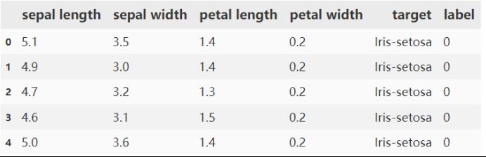
对鸢尾属植物数据分析结果如下：
先对数据进行预处理，转换成dataframe。

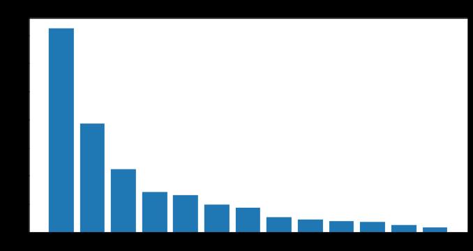
最开始使用Kmeans对四个属性进行分析，发现得出的准确率只有0.8933，这个准确率并不是很高，于是想出了先用主成分分析PCA看一下各个属性对不同类别的影响。

发现四个属性中，选用两个属性PC1和PC2更加好一些。

发现相比较来说，主成分分析好像对Kmean并没有什么好处。于是采用主成分分析+其他方法。
以KNN为：

发现PCA+KNN的效果是最为明显的，准确率直接达到了0.95。综上，PCA+KNN的方法更加适合鸢尾属植物数据的聚类分析。
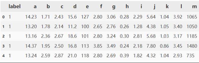
酒wine:
由于不知道各个属性是什么，我们就用a、b、c等字母来表示。

先用Kmean进行聚类，发现准确率只有0.70224，这个效果来说是非常差了，因为只有3个类别而已，于是采用KNN进行聚类，发现准确率有0.87078，虽说效果比Kmean好多了，但是也没有达到很好的效果，于是继续采用PCA+Kmean和PCA+KNN进行分析。
PCA分析如下：


可以看出用PCA+Kmean的准确率达到了0.9663，这个效果相对之前的Kmean和KNN好多了。

可以看出用PCA+KNN的准确率达到了0.9607，这个效果相对之前的Kmean和KNN也好多了，但是笔PCA+Kmean还是差点。
综上，采用PCA+Kmeand进行聚类非常好。
iris部分代码如下：

#load data
import pandas as pd
import numpy as np
data = pd.read_csv('iris_data.csv')
data.head()


# In[61]:


X = data.drop(['target','label'],axis=1)
y = data.loc[:,'label']


# In[35]:


from sklearn.preprocessing import StandardScaler
X_norm = StandardScaler().fit_transform(X)
print(X_norm)


# In[36]:


#calcualte the mean and sigma
x1_mean = X.loc[:,'sepal length'].mean()
x1_norm_mean = X_norm[:,0].mean()
x1_sigma = X.loc[:,'sepal length'].std()
x1_norm_sigma = X_norm[:,0].std()
print(x1_mean,x1_sigma,x1_norm_mean,x1_norm_sigma)


# In[37]:


#pca analysis
from sklearn.decomposition import PCA
pca = PCA(n_components=4)
X_pca = pca.fit_transform(X_norm)
#calculate the variance ratio of each principle components
var_ratio = pca.explained_variance_ratio_
print(var_ratio)


# In[71]:


from matplotlib import pyplot as plt
fig2 = plt.figure(figsize=(10,5))
plt.bar([1,2,3,4],var_ratio)
plt.xticks([1,2,3,4],['PC1','PC2','PC3','PC4'])
plt.ylabel('variance ratio of each PC')
plt.show()


# In[72]:


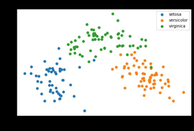
#visualize the PCA result
fig3 = plt.figure(figsize=(5,3))
setosa=plt.scatter(X_pca[:,0][y==0],X_pca[:,1][y==0])
versicolor=plt.scatter(X_pca[:,0][y==1],X_pca[:,1][y==1])
virginica=plt.scatter(X_pca[:,0][y==2],X_pca[:,1][y==2])
plt.legend((setosa,versicolor,virginica),('setosa','versicolor','virginica'))

plt.xlabel('PC1')
plt.ylabel('PC2')
plt.show()


# In[70]:


#set the model
from sklearn.cluster import KMeans
KM=KMeans(n_clusters=3,random_state=0)#分为3类  从第0个点开始
KM.fit(X)
print(X)


# In[63]:


centers=KM.cluster_centers_ 


# In[85]:


from sklearn.cluster import KMeans
KM=KMeans(n_clusters=3,random_state=0)#分为3类  从第0个点开始
KM.fit(X_pca)
centers=KM.cluster_centers_ 
from sklearn.metrics import accuracy_score
y_predict = KM.predict(X_pca)
#correct the results
y_corrected=[]
for i in y_predict:
    if i==0:
        y_corrected.append(2)
    elif i==1:
        y_corrected.append(0)
    else:
        y_corrected.append(1)
accuracy = accuracy_score(y,y_corrected)
print(accuracy)


# In[87]:


#visualize the PCA result
fig3 = plt.figure(figsize=(8,5))
setosa=plt.scatter(X_pca[:,0][y_predict==0],X_pca[:,1][y_predict==0])
versicolor=plt.scatter(X_pca[:,0][y_predict==1],X_pca[:,1][y_predict==1])
virginica=plt.scatter(X_pca[:,0][y_predict==2],X_pca[:,1][y_predict==2])
plt.legend((setosa,versicolor,virginica),('setosa','versicolor','virginica'))
plt.title("201922450902-liushipeng-PCA+Kmean accuracy:"+str(accuracy))
plt.xlabel('PC1')
plt.ylabel('PC2')
plt.show()