Hedging Strategy_TBC_有点超纲故推迟学习！

Posted 2021-03-10 sophhhie

*Catalog

1. Simulation for GBM Price Process

2. Simulation for Cost of Hedging

 

1. Simulation for GBM Price Process

　　(1) Pre-determine S0, drift mu, volatility sigma, (K, T) of call option, rebalancing period dt;

set.seed(121)
library(fOptions)
price_simulation <- function(S0, mu, sigma, rf, K, Time, dt, plots = FALSE) {
        t <- seq(0, Time, by = dt)
        N <- length(t)
        # w~N(0,1)
        w <- c(0, cumsum(rnorm(N - 1)))
        S <- S0 * exp((mu - sigma^2 / 2) * t + sigma * sqrt(dt) * w)
        delta <- rep(0, N - 1)
        call_ <- rep(0, N - 1)
        for(i in 1:(N - 1)) {
                delta[i] <- GBSGreeks(‘Delta‘, ‘c‘, S[i], K, Time - t[i],
                                      rf, rf, sigma)
                call_[i] <- GBSOption(‘c‘, S[i], K, Time - t[i],
                                      rf, rf, sigma)@price
        }
        if(plots){
                dev.new(width = 30, height = 10)
                par(mfrow = c(1, 3))
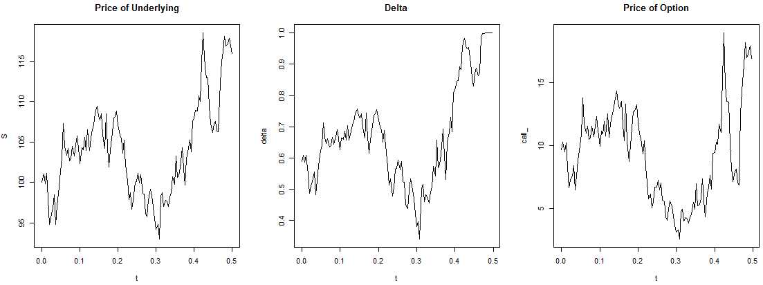
                plot(t, S, type = ‘l‘, main = ‘Price of Underlying‘)
                plot(t[-length(t)], delta, type = ‘l‘, main = ‘Delta‘,
                     xlab = ‘t‘)
                plot(t[-length(t)], call_, type = ‘l‘, main = ‘Price of Option‘,
                     xlab = ‘t‘)
        }
}
price_simulation(100, 0.2, 0.3, 0.05, 100, 0.5, 1/250, plots = TRUE)

　　(2) Analysis:

　　　　/Delta converges to 1 and it follows the stock‘s fluctuations! If spot price goes up, prob to exercise call option also goes up, so we have to buy more stocks in order to replicate the call; if spot price falls, we sell stocks. Thus, price of option derives from the cost of hedging (PV of cumulative net costs(amount to buy shares + interest of financing the position) of buying and selling stock necessary to hedge the position);

　　　　/Stock price quickly arrives at ITM level of 100, so option is exercised at maturity;

 

 

 2. Simulation for Cost of Hedging

　　(1) First calculate cost of hedging for the written call:

cost_simulation = function(S0, mu, sigma, rf, K, Time, dt){
        t <- seq(0, Time, by = dt)
        N <- length(t)
        W <- c(0, cumsum(rnorm(N - 1)))
        S <- S0 * exp((mu - sigma^2 / 2) * t + sigma * sqrt(dt) * W)
        delta <- rep(0, N - 1)
        call_ <- rep(0, N - 1)
        for(i in 1 : (N - 1)){
                delta[i] <- GBSGreeks(‘Delta‘, ‘c‘, S[i], K, Time - t[i],
                                      rf, rf, sigma)
                call_[i] <- GBSOption(‘c‘, S[i], K, Time - t[i],
                                      rf, rf, sigma)@price
        }
        share_cost <- rep(0, N - 1)
        interest_cost <- rep(0, N - 1)
        total_cost <- rep(0, N - 1)
        share_cost[1] <- S[1] * delta[1]
        interest_cost[1] <- (exp(rf * dt) - 1) * share_cost[1]
        total_cost[1] <- share_cost[1] + interest_cost[1]
        for(i in 2:(N - 1)){
                share_cost[i] <- (delta[i] - delta[i - 1]) * S[i]
                interest_cost[i] <- (total_cost[i - 1] + share_cost[i]) * (exp(rf * dt) - 1)
                total_cost[i] <- total_cost[i - 1] + interest_cost[i] + share_cost[i]
        }
        c = max(S[N] - K, 0)
        cost = c - delta[N - 1] * S[N] + total_cost[N - 1]
        return(cost * exp(-Time * rf))
}

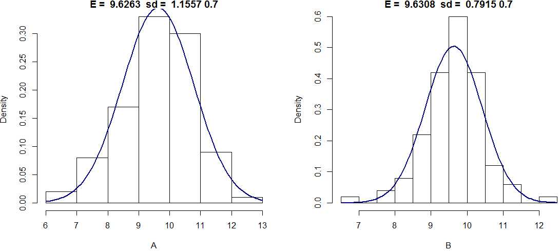
　　(2) Draw two strategies:

A = rep(0, 100)
for(i in 1:100){
        A[i] = cost_simulation(100, .2, .3, .05, 100, .5, 1/52)
}
B = rep(0, 100)
for(i in 1:100){
        B[i] = cost_simulation(100, .2, .3, .05, 100, .5, 1/250)
}
dev.new(width = 20, height = 10)
par(mfrow = c(1, 2))
hist(A, freq = F, main = paste(‘E = ‘, round(mean(A), 4), ‘ sd = ‘,
                               round(sd(A), 4), xlim = c(6, 14, ylim = c(0, .7))))
curve(dnorm(x, mean = mean(A), sd = sd(A)), col = ‘darkblue‘,
      lwd = 2, add = T, yaxt = ‘n‘)
hist(B, freq = F, main = paste(‘E = ‘, round(mean(B), 4), ‘ sd = ‘,
                               round(sd(B), 4), xlim = c(6, 14, ylim = c(0, .7))))
curve(dnorm(x, mean = mean(B), sd = sd(B)), col = ‘darkblue‘,
      lwd = 2, add = T, yaxt = ‘n‘)

/A is weekly hedging, B is daily rebalancing;

/The more frequent rebalancing, sd of cost of hedging be reduced;

/expected value also lower, 9.6308 < 9.6263, and closer to BS price.

 

 

 3.