《DSP using MATLAB》Problem 7.11

Posted 2021-02-11 ky027wh-sx

代码：

%% ++++++++++++++++++++++++++++++++++++++++++++++++++++++++++++++++++++++++++++++++
%%            Output Info about this m-file
fprintf(‘
***********************************************************
‘);
fprintf(‘        <DSP using MATLAB> Problem 7.11 

‘);

banner();
%% ++++++++++++++++++++++++++++++++++++++++++++++++++++++++++++++++++++++++++++++++

% bandpass
ws1 = 0.3*pi; wp1 = 0.4*pi; wp2 = 0.5*pi; ws2 = 0.6*pi; As = 50; Rp = 0.5;
tr_width = min((wp1-ws1), (ws2-wp2));
M = ceil(6.6*pi/tr_width) + 1;                 % Hamming Window
fprintf(‘
Filter Length is %d.
‘, M);


n = [0:1:M-1]; wc1 = (ws1+wp1)/2; wc2 = (wp2+ws2)/2;

%wc = (ws + wp)/2,                    % ideal LPF cutoff frequency

hd = ideal_lp(wc2, M) - ideal_lp(wc1, M); 
w_hamm = (hamming(M))‘;  h = hd .* w_hamm;
[db, mag, pha, grd, w] = freqz_m(h, [1]);  delta_w = 2*pi/1000;
[Hr,ww,P,L] = ampl_res(h);

Rp = -(min(db(wp1/delta_w+1 :1: wp2/delta_w)));     % Actual Passband Ripple
fprintf(‘
Actual Passband Ripple is %.4f dB.
‘, Rp);

As = -round(max(db(ws2/delta_w+1 : 1 : 501)));        % Min Stopband attenuation
fprintf(‘
Min Stopband attenuation is %.4f dB.
‘, As);

[delta1, delta2] = db2delta(Rp, As)

% Plot

figure(‘NumberTitle‘, ‘off‘, ‘Name‘, ‘Problem 7.11 ideal_lp Method‘)
set(gcf,‘Color‘,‘white‘); 

subplot(2,2,1); stem(n, hd); axis([0 M-1 -0.3 0.3]); grid on;
xlabel(‘n‘); ylabel(‘hd(n)‘); title(‘Ideal Impulse Response‘);

subplot(2,2,2); stem(n, w_hamm); axis([0 M-1 0 1.1]); grid on;
xlabel(‘n‘); ylabel(‘w(n)‘); title(‘Hamming Window‘);

subplot(2,2,3); stem(n, h); axis([0 M-1 -0.3 0.3]); grid on;
xlabel(‘n‘); ylabel(‘h(n)‘); title(‘Actual Impulse Response‘);

subplot(2,2,4); plot(w/pi, db); axis([0 1 -100 10]); grid on;
set(gca,‘YTickMode‘,‘manual‘,‘YTick‘,[-90,-51,0]);
set(gca,‘YTickLabelMode‘,‘manual‘,‘YTickLabel‘,[‘90‘;‘51‘;‘ 0‘]);
set(gca,‘XTickMode‘,‘manual‘,‘XTick‘,[0,0.3,0.4,0.5,0.6,1]);
xlabel(‘frequency in pi units‘); ylabel(‘Decibels‘); title(‘Magnitude Response in dB‘);


figure(‘NumberTitle‘, ‘off‘, ‘Name‘, ‘Problem 7.11 h(n) ideal_lp Method‘)
set(gcf,‘Color‘,‘white‘); 

subplot(2,2,1); plot(w/pi, db); grid on; %axis([0 1 -100 10]); 
xlabel(‘frequency in pi units‘); ylabel(‘Decibels‘); title(‘Magnitude Response in dB‘);
set(gca,‘YTickMode‘,‘manual‘,‘YTick‘,[-90,-51,0])
set(gca,‘YTickLabelMode‘,‘manual‘,‘YTickLabel‘,[‘90‘;‘51‘;‘ 0‘]);
set(gca,‘XTickMode‘,‘manual‘,‘XTick‘,[0,0.3,0.4,0.5,0.6,1,1.4,1.5,1.6,1.7,2]);

subplot(2,2,3); plot(w/pi, mag); grid on; %axis([0 1 -100 10]); 
xlabel(‘frequency in pi units‘); ylabel(‘Absolute‘); title(‘Magnitude Response in absolute‘);
set(gca,‘XTickMode‘,‘manual‘,‘XTick‘,[0,0.3,0.4,0.5,0.6,1,1.4,1.5,1.6,1.7,2]);
set(gca,‘YTickMode‘,‘manual‘,‘YTick‘,[0.0,0.5,1.0])


subplot(2,2,2); plot(w/pi, pha); grid on; %axis([0 1 -100 10]); 
xlabel(‘frequency in pi units‘); ylabel(‘Rad‘); title(‘Phase Response in Radians‘);
subplot(2,2,4); plot(w/pi, grd*pi/180);  grid on; %axis([0 1 -100 10]); 
xlabel(‘frequency in pi units‘); ylabel(‘Rad‘); title(‘Group Delay‘);


figure(‘NumberTitle‘, ‘off‘, ‘Name‘, ‘Problem 7.11 h(n)‘)
set(gcf,‘Color‘,‘white‘); 

plot(ww/pi, Hr); grid on; %axis([0 1 -100 10]); 
xlabel(‘frequency in pi units‘); ylabel(‘Hr‘); title(‘Amplitude Response‘);
set(gca,‘YTickMode‘,‘manual‘,‘YTick‘,[-delta2,0,delta2,1 - delta1,1, 1 + delta1])
%set(gca,‘YTickLabelMode‘,‘manual‘,‘YTickLabel‘,[‘90‘;‘45‘;‘ 0‘]);
%set(gca,‘XTickMode‘,‘manual‘,‘XTick‘,[0,0.2,0.35,0.55,0.75,1,1.2,1.55,2]);

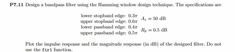
　　运行结果：

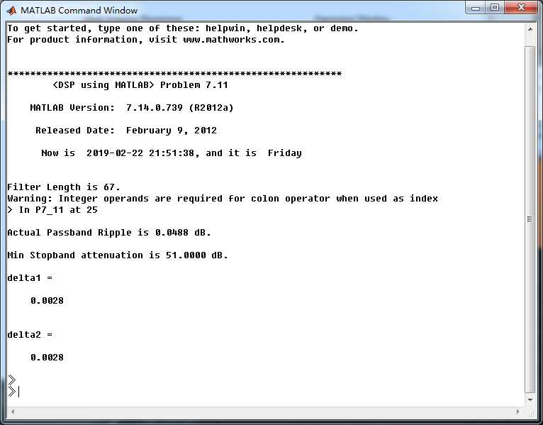
        阻带最小衰减51dB，满足设计要求。

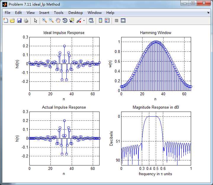
         Hamming窗截断的滤波器脉冲响应，其幅度响应（dB和Absolute单位）、相位响应和群延迟

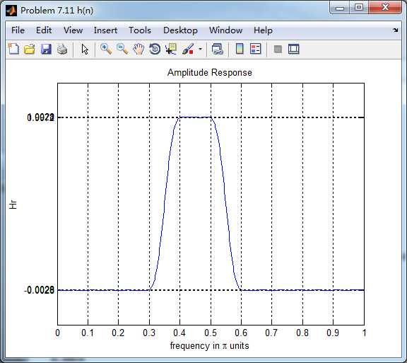
        振幅响应

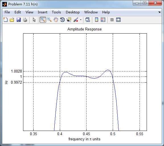
        带通部分

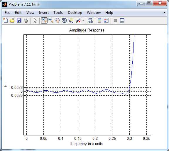
        阻带部分