First Steps with TensorFlow代码解析

Posted 2021-01-06 woods-bagnzhu

注：本文的内容基本上都摘自tensorflow的官网，只不过官网中的这部分内容在国内访问不了，所以我只是当做一个知识的搬运工，同时梳理了一遍，方便大家查看。本文相关内容地址如下：

https://developers.google.cn/machine-learning/crash-course/ml-intro

 

一、first_steps_with_tensor_flow可运行代码

以下是tensorflow官网中first_steps_with_tensor_flow.py的完整可运行代码，直接复制编译就可以出结果。代码如下：

import math
from IPython import display
from matplotlib import cm
from matplotlib import gridspec
from matplotlib import pyplot as plt
import numpy as np
import pandas as pd
from sklearn import metrics
import tensorflow as tf
from tensorflow.python.data import Dataset


def my_input_fn(features, targets, batch_size = 1, shuffle=True, num_epochs = None):
  
    # Convert pandas data into a dict of np arrays.
    features = {key:np.array(value) for key,value in dict(features).items()}                                           
  
    # Construct a dataset, and configure batching/repeating
    ds = Dataset.from_tensor_slices((features,targets)) # warning: 2GB limit
    ds = ds.batch(batch_size).repeat(num_epochs)
    
    # Shuffle the data, if specified
    if shuffle:
      ds = ds.shuffle(buffer_size=10000)
    
    # Return the next batch of data
    features, labels = ds.make_one_shot_iterator().get_next()
    return features, labels



def train_model(learning_rate, steps, batch_size, input_feature="total_rooms"):

      periods = 10
      steps_per_period = steps / periods
      # 第 1 步：定义特征并配置特征列
      my_feature = input_feature
      my_feature_data = california_housing_dataframe[[my_feature]]
      # Create feature columns
      feature_columns = [tf.feature_column.numeric_column(my_feature)]

      # 第 2 步：定义目标
      my_label = "median_house_value"
      targets = california_housing_dataframe[my_label]


      # 第 4 步：定义输入函数
      # Create input functions
      training_input_fn = lambda:my_input_fn(my_feature_data, targets, batch_size=batch_size)
      prediction_input_fn = lambda: my_input_fn(my_feature_data, targets, num_epochs=1, shuffle=False)

      # 第 3 步：配置 LinearRegressor 线性回归器
      # Create a linear regressor object.
      my_optimizer = tf.train.GradientDescentOptimizer(learning_rate=learning_rate)
      my_optimizer = tf.contrib.estimator.clip_gradients_by_norm(my_optimizer, 5.0)
      linear_regressor = tf.estimator.LinearRegressor(
          feature_columns=feature_columns,
          optimizer=my_optimizer
      )

      # Set up to plot the state of our model‘s line each period.
      plt.figure(figsize=(15, 6))
      plt.subplot(1, 2, 1)
      plt.title("Learned Line by Period")
      plt.ylabel(my_label)
      plt.xlabel(my_feature)
      sample = california_housing_dataframe.sample(n=300)
      plt.scatter(sample[my_feature], sample[my_label])
      colors = [cm.coolwarm(x) for x in np.linspace(-1, 1, periods)]

      # Train the model, but do so inside a loop so that we can periodically assess
      # loss metrics.
      print("Training model...")
      print("RMSE (on training data):")

      root_mean_squared_errors = []

      for period in range (0, periods):
            # 第 5 步：训练模型
            # Train the model, starting from the prior state.
            linear_regressor.train(
                input_fn=training_input_fn,
                steps=steps_per_period
            )
            # 第 6 步：评估模型
            # Take a break and compute predictions.
            predictions = linear_regressor.predict(input_fn=prediction_input_fn)
            predictions = np.array([item[‘predictions‘][0] for item in predictions])

            # Compute loss.
            root_mean_squared_error = math.sqrt(
                metrics.mean_squared_error(predictions, targets))
            # Occasionally print the current loss.
            print("  period %02d : %0.2f" % (period, root_mean_squared_error))



            # Add the loss metrics from this period to our list.
            root_mean_squared_errors.append(root_mean_squared_error)
            # Finally, track the weights and biases over time.
            # Apply some math to ensure that the data and line are plotted neatly.
            y_extents = np.array([0, sample[my_label].max()])

            weight = linear_regressor.get_variable_value(‘linear/linear_model/%s/weights‘ % input_feature)[0]
            bias = linear_regressor.get_variable_value(‘linear/linear_model/bias_weights‘)

            x_extents = (y_extents - bias) / weight
            x_extents = np.maximum(np.minimum(x_extents,
                                              sample[my_feature].max()),
                                   sample[my_feature].min())
            y_extents = weight * x_extents + bias

            plt.plot(x_extents, y_extents, color = colors[period])


      print("Model training finished.")


      # Output a graph of loss metrics over periods.
      plt.subplot(1, 2, 2)
      plt.ylabel(‘RMSE‘)
      plt.xlabel(‘Periods‘)
      plt.title("Root Mean Squared Error vs. Periods")
      plt.tight_layout()
      plt.plot(root_mean_squared_errors)
      plt.show()

      # Output a table with calibration data.
      calibration_data = pd.DataFrame()
      calibration_data["predictions"] = pd.Series(predictions)
      calibration_data["targets"] = pd.Series(targets)
      display.display(calibration_data.describe())

      print("Final RMSE (on training data): %0.2f" % root_mean_squared_error)


tf.logging.set_verbosity(tf.logging.ERROR)
pd.options.display.max_rows = 10
pd.options.display.float_format = ‘{:.1f}‘.format

california_housing_dataframe = pd.read_csv(
  "E://woodsfile//machine learning//Tensorflow实战代码//tensorflow使用步骤//california_housing_train.csv",
   sep=",")

## 对数据进行随机化处理
california_housing_dataframe = california_housing_dataframe.reindex(
  np.random.permutation(california_housing_dataframe.index))

california_housing_dataframe["median_house_value"] /= 1000.0

# 输出关于各列的一些实用统计信息快速摘要：样本数、均值、标准偏差、最大值、最小值和各种分位数
california_housing_dataframe.describe()


train_model(
    learning_rate=0.00002,
    steps=500,
    batch_size=5
)

运行结果如下：

 

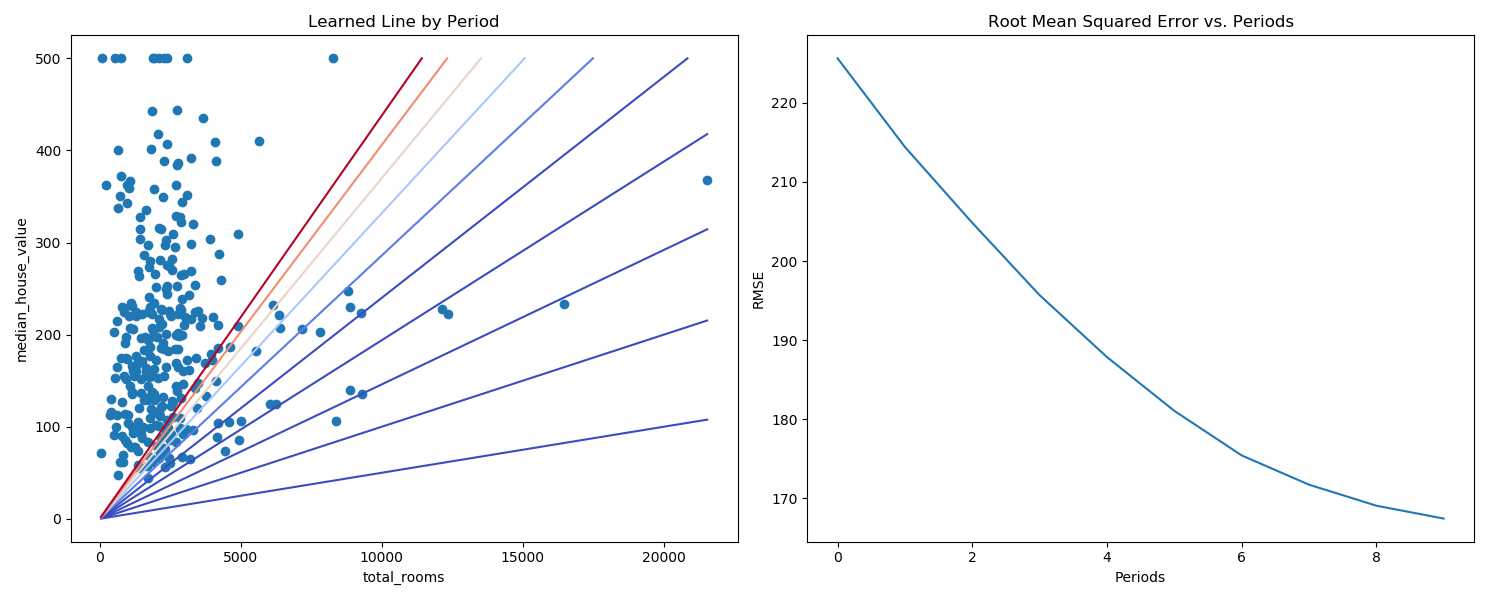
此程序实现输入房间总数（total_rooms），预测得到房子的价格（median_house_vaule）。

左边figure，每训练一次，就画一条预测函直线，共预测了十次。右边figure表示了每次预测的RMSE的值。

 

上述代码中关于california房屋统计情况的数据集请在我的百度网盘上下载，地址如下：

https://pan.baidu.com/s/1A-EbKXRIP7q_5uraRmbXxw

（注：下面一小节的代码是第一部分的详细步骤，代码不完全一致，基本步骤是一样的。）

 

二、使用tensorflow的基本步骤

使用tensorflow有以下几个基本步骤：

1. 定义特征并配置特征列
2. 定义目标(label)
3. 配置线性回归模型
4. 定义输入函数
5. 训练模型
6. 评估模型

1、定义特征并配置特征列

本例中只采用了数据列表中“total_rooms”这一个特征，并将这些数据转化为数值。

以下代码从california_housing_dataframe中提取total_rooms数据，并使用numeric_column将数据指定为数值。

1 # Define the input feature: total_rooms.
2 # 只提取一个特征值：total_rooms
3 my_feature = california_housing_dataframe[["total_rooms"]]
4 
5 # 将total_rooms列中的数据转化为数值，为一维数组
6 feature_columns = [tf.feature_column.numeric_column("total_rooms")]

 

2、定义目标(label)

接下来定义目标即median_house_value，同样从california_housing_dataframe提取。

1 # Define the label.
2 targets = california_housing_dataframe["median_house_value"]

 

3、配置线性回归模型

接下来我们使用线性回归模型(LinearRegressor)，并使用随机梯度下降法(SGD)训练该模型。learning_rate参数用来控制梯度补偿大小。为了安全起见，程序中通过clip_gradients_by_norm将梯度裁剪应用到我们的优化器。梯度裁剪可确保梯度大小在训练期间不会变得过大，梯度过大将会导致梯度下降算法失败。

# Use gradient descent as the optimizer for training the model.
my_optimizer = tf.train.GradientDescentOptimizer(learning_rate=0.0000001)

#这一步使用了梯度裁剪，保证梯度大小在训练期间不会变得过大，梯度过大导致梯度下降法失败
my_optimizer = tf.contrib.estimator.clip_gradients_by_norm(my_optimizer, 5.0) 

# Configure the linear regression model with our feature columns and optimizer.
# Set a learning rate of 0.0000001 for Gradient Descent.
linear_regressor = tf.estimator.LinearRegressor(
    feature_columns = feature_columns,
    optimizer = my_optimizer
)

 

4、定义输入函数

要将california住房数据导入LinearRegressor，我们需要定义一个输入函数。这个函数的作用是告诉TensorFlow如何对数据进行预处理，以及在模型训练期间如何批处理、随机处理和重复数据。

程序中，首先将Pandas特征数据转换成Numpy数组字典。然后，我们可以使用TensorFlow Dataset API根据我们的数据构建Dataset对象，并将数据拆分成大小为batch_size的多批数据，以按照指定周期数(num_epochs)进行重复。最后，输入函数会为该数据集构建一个迭代器，并向LinearRegressor返回下一批数据。

注意：

• 如果将默认值num_epochs=None传递到repeat()，输入数据会无限期循环。
• 如果shuffle这只为true，则我们会对数据进行随机处理，以便数据在训练期间以随机方式传递到模型。buffer_size参数会指定shuffle随机抽样的数据集大小。

def my_input_fn(features, targets, batch_size=1, shuffle=True, num_epochs=None):

    # Convert pandas data into a dict of np arrays.
    features = {key:np.array(value) for key,value in dict(features).items()}                                           
     
    # Construct a dataset, and configure batching/repeating
    ds = Dataset.from_tensor_slices((features,targets)) # warning: 2GB limit
    ds = ds.batch(batch_size).repeat(num_epochs)
    
    # Shuffle the data, if specified
    if shuffle:
      ds = ds.shuffle(buffer_size=10000)
    
    # Return the next batch of data
    features, labels = ds.make_one_shot_iterator().get_next()
    return features, labels

 

5、训练模型

接下来在linear_regressor上调用train()来训练模型。我们会将my_inout_fn封装在lambda中，以便可以将my_feature和target作为参数传入。

# 训练steps = 100步
_ = linear_regressor.train(
    input_fn = lambda:my_input_fn(my_feature, targets),
    steps=100
    )

 

6、评估模型

我们基于该训练数据做一侧预测，看看我们的模型在训练期间与这些数据的拟合情况。(对代码有疑问的话，代码上方的注释都给出了很明确的说明。注释都很小并且都是英文，往往容易被我们忽视，别这样做。)

# Create an input function for predictions.
# Note: Since we‘re making just one prediction for each example, we don‘t 
# need to repeat or shuffle the data here.
prediction_input_fn =lambda: my_input_fn(my_feature, targets, num_epochs=1, shuffle=False)
 
# Call predict() on the linear_regressor to make predictions.
predictions = linear_regressor.predict(input_fn=prediction_input_fn)
 
# Format predictions as a NumPy array, so we can calculate error metrics.
predictions = np.array([item[‘predictions‘][0] for item in predictions])
 
# Print Mean Squared Error and Root Mean Squared Error.
mean_squared_error = metrics.mean_squared_error(predictions, targets)
root_mean_squared_error = math.sqrt(mean_squared_error)
print("Mean Squared Error (on training data): %0.3f" % mean_squared_error)
print("Root Mean Squared Error (on training data): %0.3f" % root_mean_squared_error) 

由于均方误差(MSE)很难解读，我们经常查看的是均方根误差（RMSE）。RMSE是一个很好的特性可以在与原目标相同的规模下解读。

那上面的预测效果到底如何呢？我们可以通过查看总体摘要的统计信息进行查看，代码如下：

calibration_data = pd.DataFrame()
calibration_data["predictions"] = pd.Series(predictions)
calibration_data["targets"] = pd.Series(targets)
calibration_data.describe()
print(calibration_data.describe())