线性回归

Posted 2020-12-26 qinhao2

创建线性回归模型

import sklearn.linear_model as lm

sklearn.linear_model.LinearRegression()->线性回归器
线性回归器.fit(输入样本, 输出标签)
线性回归器.predict(输入样本)->预测输出标签

4.94,4.37
-1.58,1.7
-4.45,1.88
-6.06,0.56
-1.22,2.23
-3.55,1.53
0.36,2.99
-3.24,0.48
1.31,2.76
2.17,3.99
2.94,3.25
-0.92,2.27
-0.91,2.0
1.24,4.75
1.56,3.52
-4.14,1.39
3.75,4.9
4.15,4.44
0.33,2.72
3.41,4.59
2.27,5.3
2.6,3.43
1.06,2.53
1.04,3.69
2.74,3.1
-0.71,2.72
-2.75,2.82
0.55,3.53
-3.45,1.77
1.09,4.61
2.47,4.24
-6.35,1.0
1.83,3.84
-0.68,2.42
-3.83,0.67
-2.03,1.07
3.13,3.19
0.92,4.21
4.02,5.24
3.89,3.94
-1.81,2.85
3.94,4.86
-2.0,1.31
0.54,3.99
0.78,2.92
2.15,4.72
2.55,3.83
-0.63,2.58
1.06,2.89
-0.36,1.99

线性回归数据集

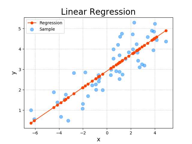
 1 import numpy as np
 2 import sklearn.linear_model as lm
 3 import sklearn.metrics as sm
 4 import matplotlib.pyplot as mp
 5 
 6 # x,y用来装x,y上的点
 7 x, y = [], []
 8 with open(‘../ML/data/single.txt‘, ‘r‘) as f:
 9     for line in f.readlines():
10         data = [float(substr) for substr in line.split(‘,‘)]
11         x.append(data[:-1])
12         y.append(data[-1])
13 
14 x = np.array(x)
15 y = np.array(y)
16 # print(x)
17 # 创建线性回归模型器
18 model = lm.LinearRegression()
19 # 导入数据
20 model.fit(x, y)
21 # 生成预测点
22 pred_y = model.predict(x)
23 
24 # 画训练集的图像
25 mp.figure(‘Linear Regression‘, facecolor=‘lightgray‘)
26 mp.title(‘Linear Regression‘, fontsize=20)
27 mp.xlabel(‘x‘, fontsize=14)
28 mp.ylabel(‘y‘, fontsize=14)
29 mp.tick_params(labelsize=10)
30 mp.grid(linestyle=‘:‘)
31 mp.scatter(x, y, c=‘dodgerblue‘, alpha=0.55, s=60, label=‘Sample‘)
32 
33 # 画线性回归的图像
34 # argsort()函数是将x中的元素从小到大排列，提取其对应的index(索引)，然后输出到y。
35 sorted_indices = x.T[0].argsort()
36 mp.plot(x[sorted_indices], pred_y[sorted_indices],
37         ‘o-‘, c=‘orangered‘, label=‘Regression‘)
38 
39 mp.legend()
40 mp.show()

线性回归代码

保存模型

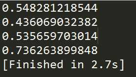
 1 import numpy as np
 2 import sklearn.linear_model as lm
 3 import sklearn.metrics as sm
 4 import matplotlib.pyplot as mp
 5 # 导入pickle
 6 import pickle
 7 
 8 x, y = [], []
 9 with open(‘../ML/data/single.txt‘, ‘r‘) as f:
10     for line in f.readlines():
11         data = [float(substr) for substr in line.split(‘,‘)]
12         x.append(data[:-1])
13         y.append(data[-1])
14 
15 x = np.array(x)
16 y = np.array(y)
17 model = lm.LinearRegression()
18 model.fit(x, y)
19 pred_y = model.predict(x)
20 
21 # sklearn中的回归器性能评估方法
22 
23 # 平均绝对值误差（mean_absolute_error）
24 print(sm.mean_absolute_error(y, pred_y))
25 # 均方差（mean-squared-error）
26 print(sm.mean_squared_error(y, pred_y))
27 # 中值绝对误差（Median absolute error）
28 print(sm.median_absolute_error(y, pred_y))
29 # R2 决定系数（拟合优度）
30 print(sm.r2_score(y, pred_y))
31 
32 # 保存模型
33 with open(‘linear.pkl‘, ‘wb‘) as f:
34     pickle.dump(model, f)
35 
36 mp.figure(‘Linear Regression‘, facecolor=‘lightgray‘)
37 mp.title(‘Linear Regression‘, fontsize=20)
38 mp.xlabel(‘x‘, fontsize=14)
39 mp.ylabel(‘y‘, fontsize=14)
40 mp.tick_params(labelsize=10)
41 mp.grid(linestyle=‘:‘)
42 mp.scatter(x, y, c=‘dodgerblue‘, alpha=0.55, s=60, label=‘Sample‘)
43 
44 sorted_indices = x.T[0].argsort()
45 mp.plot(x[sorted_indices], pred_y[sorted_indices],
46         ‘o-‘, c=‘orangered‘, label=‘Regression‘)
47 
48 mp.legend()
49 mp.show()

保存模型及回归器性能评估

 导入模型

 1 import numpy as np
 2 import sklearn.linear_model as lm
 3 import sklearn.metrics as sm
 4 import matplotlib.pyplot as mp
 5 import pickle
 6 
 7 x, y = [], []
 8 with open(‘../ML/data/single.txt‘, ‘r‘) as f:
 9     for line in f.readlines():
10         data = [float(substr) for substr in line.split(‘,‘)]
11         x.append(data[:-1])
12         y.append(data[-1])
13 x = np.array(x)
14 y = np.array(y)
15 
16 # 导入模型
17 with open(‘linear.pkl‘, ‘rb‘) as f:
18     model = pickle.load(f)
19 pred_y = model.predict(x)
20 
21 mp.figure(‘Linear Regression‘, facecolor=‘lightgray‘)
22 mp.title(‘Linear Regression‘, fontsize=20)
23 mp.xlabel(‘x‘, fontsize=14)
24 mp.ylabel(‘y‘, fontsize=14)
25 mp.tick_params(labelsize=10)
26 mp.grid(linestyle=‘:‘)
27 mp.scatter(x, y, c=‘dodgerblue‘, alpha=0.55, s=60, label=‘Sample‘)
28 
29 sorted_indices = x.T[0].argsort()
30 mp.plot(x[sorted_indices], pred_y[sorted_indices],
31         ‘o-‘, c=‘orangered‘, label=‘Regression‘)
32 
33 mp.legend()
34 mp.show()

导入模型