0005.有监督学习之逻辑回归(Logistic回归)
Posted lxinghua
tags:
篇首语:本文由小常识网(cha138.com)小编为大家整理,主要介绍了0005.有监督学习之逻辑回归(Logistic回归)相关的知识,希望对你有一定的参考价值。
一、逻辑回归概述
分类计数是机器学习和数据挖掘应用中的重要组成部分。在数据科学中,大约70%的问题属于分类问题。解决分类问题也有很多种,比如:k-近邻算法,使用距离计算来实现分类;决策树,通过构建直观易懂的树来实现分类;朴素贝叶斯,使用概率论构建分类器。这里要讲的是Logistic回归,它是一种很常见的用来解决二元分类问题的回归方法,它主要是通过寻找最优参数来正确地分类原始数据。
1. Logistic Regression
逻辑回归(Logistic Regression,简称LR),其实是一个很有误导性的概念,虽然它的名字中带有“回归”两个字,但是它最擅长处理的却是分类问题。LR分类器适用于各项广义上的分类任务,录入:评论信息的正负情感分析(二分类)、用户点击率(二分类)、用户违约信息预测(二分类)、垃圾邮件检测(二分类)、疾病预测(二分类)、用户等级分类(多分类)等场景。这里主要讨论的是 二分类问题。
1.1 线性回归
提到逻辑回归我们不得不提一下线性回归,逻辑回归和线性回归属于广义线性模型,逻辑回归就是用线性回归模型的预测值去拟合真实标签的对数几率(一个事件的几率(odds)是指该事件发生的概率与不发生的概率之比,如果该事件发生的概率为P,那么该事件的几率是P/(1-P),对数几率就是log(P/(1-P))。
逻辑回归和线性回归本质上都是得到一条直线,不同的是,线性回归的直线是尽可能去拟合输入变量X的分析,使得训练集中所有样本点到直线的距离最短;而逻辑回归的直线是尽可能去拟合决策边界,使得训练集样本中的样本点尽可能分离开。因此,两者的目的是不同的。
线性回归方程: y = wx + b
此处,y是因变量,x为自变量。在机器学习中y是标签,x是特征。
1.2 Sigmoid函数
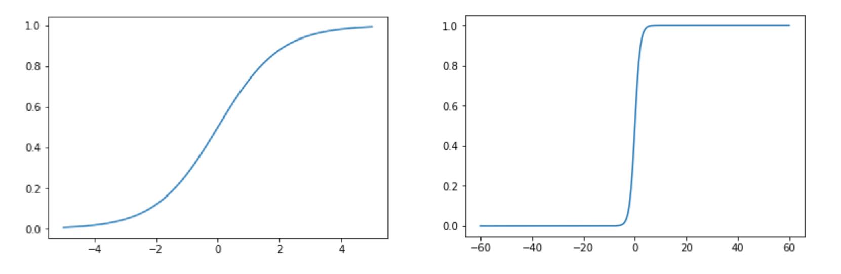
我们想要的函数应该是:能接受所有的输入然后预测出类别。例如在二分类的情况下,函数能输出0或1.那拥有这类性质的函数称为海维赛德阶跃函数(Heaviside stop function),又称之为单位阶跃函数。如图所示:

单位阶跃函数的问题在于:在0点位置该函数从0瞬间跳跃到1,这个孙坚跳跃过程很难处理(不好求导)。幸运的是,Sigmoid函数也有类似的性质,且数学上更容易处理。
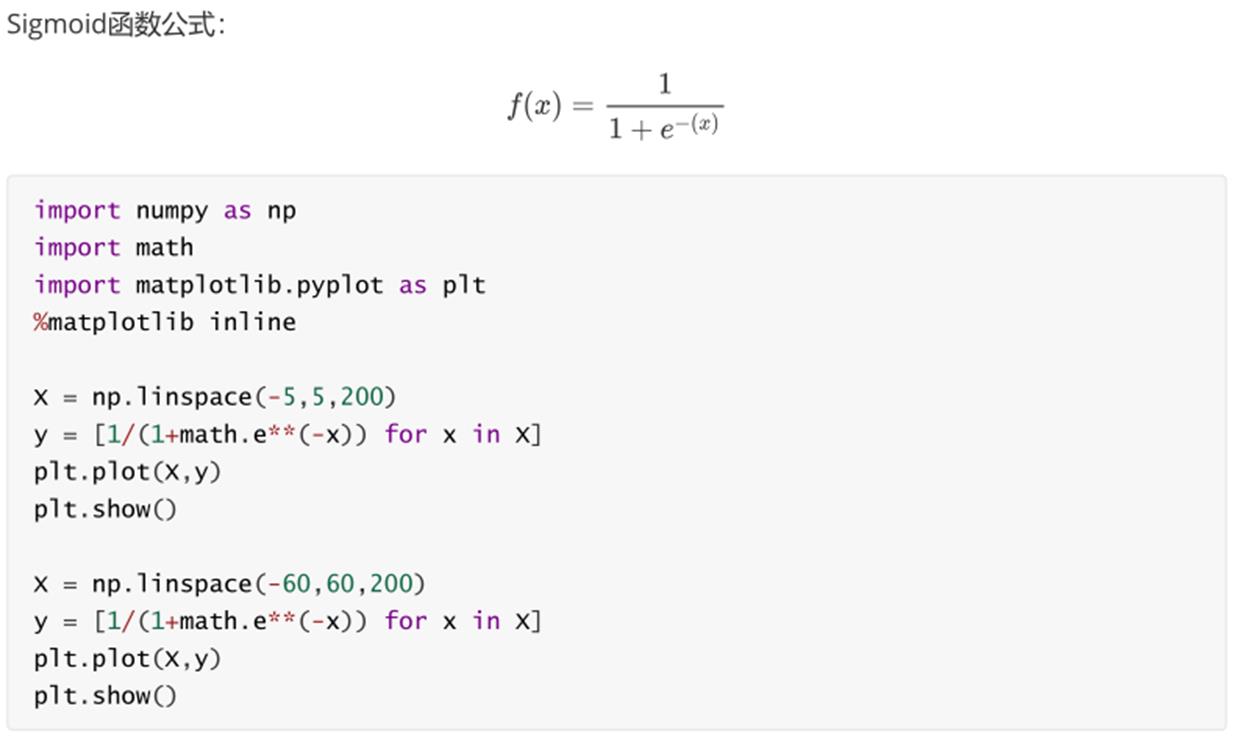
下图给出了Sigmoid函数在不同坐标尺度下的两条曲线。当x为0时, Sigmoid函数值为0.5. 随着x的增大,对应的函数值将逼近于1;而随着x的减少,函数值逼近于0. 所以Sigoin函数值域为(0,1),注意这是开区间,它仅无限接近0和1.如果横坐标刻度足够大,Sigmoid函数看起来就很想一个阶跃函数。
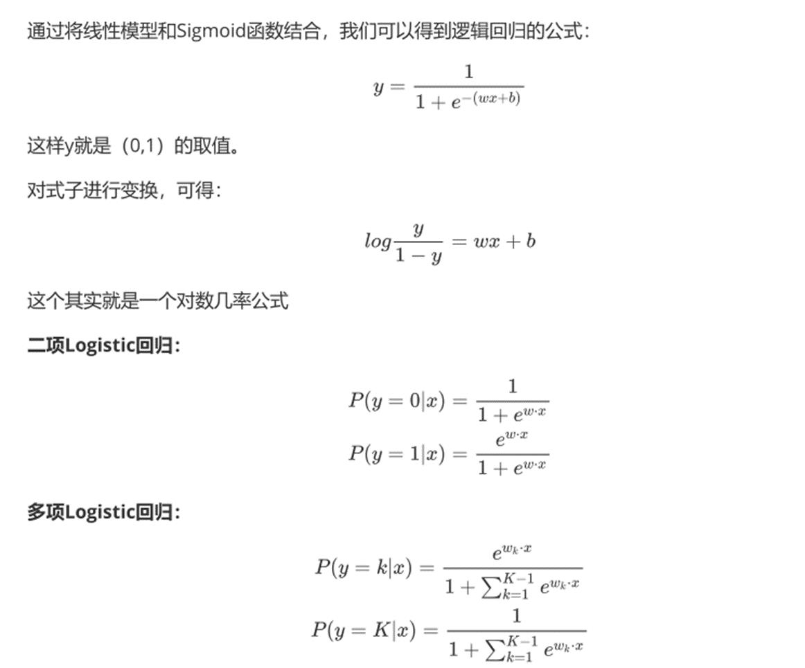
1.3 逻辑回归
1.4 LR与线性回归的区别
逻辑回归和线性回归是两类模型,逻辑回归是分类模型,线性回归是回归模型。
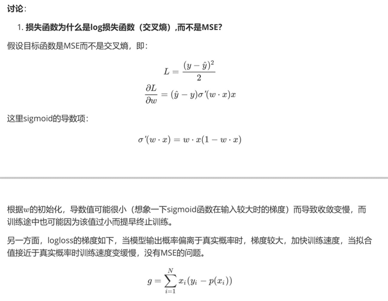
2. LR的损失函数
损失函数,通俗讲,就是衡量真实值和预测值之间差距的函数。所以函数越小,模型就越好。在这里,最小损失是0。
LR损失函数为:

可以看一下这个函数的图像:
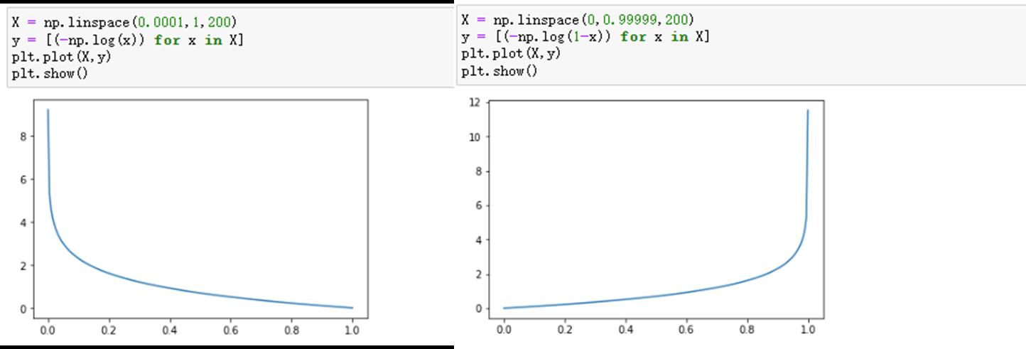

不过当损失过于小的时候,也就是模型能够拟合绝大部分的数据,这时候就容易出现过拟合。为了防止过拟合,我们会引入正则化。
3. LR正则化
3.1 L1 正则化
Lasso回归,相当于为模型添加了这样一个先验条件:w服从零均值拉普拉斯分析。

等价于原始的cross-entropy后面加上了L1正则,因此L1正则的本质其实是为模型增加了“模型参数服从零均值拉普拉斯分析”这一先验条件。
3.2 L2正则化
Ridge回归,相当于为模型添加了这样一个先验条件:w服从零均值正态分布。
等价于原始的cross-entropy后面加上了L2正则,因此L2正则的本质其实是为模型增加了“模型参数服从零均值正态分布”这一先验条件。
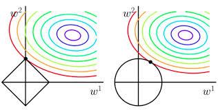
3.3 L1正则化和L2正则化的区别
1. 两者引入的关于模型参数的先验条件不一样,L1是拉普拉斯分布,L2是正态分布;
2. L1偏向于使模型参数变得稀疏(但实际上并不那么容易),L2 偏向于使模型每一个参数都很小,但是更加稠密,从而防止过拟合。
为什么L1偏向于稀疏,L2偏向于稠密呢?
看下面两张图,每一个圆表示loss的等高线,即在该圆上loss都是相同的,可以看到L1更容易在坐标轴上达到,而L2则容易在象限里达到。
4. RL损失函数求解
4.1 基于对数似然损失函数
4.2 基于极大似然估计

二、梯度下降法
由于极大似然函数无法直接求解,所以在机器学习算法中,在最下化损失函数时,可以通过梯度下降法来一步步的迭代求解,得到最下化的损失函数和模型参数值。
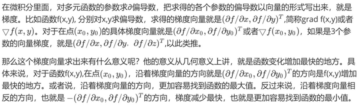
1. 梯度
2. 梯度下降的直观解释
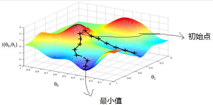
首先来看看梯度下降的一个直观的解释。比如我们在一座大山上的某处位置,由于我们不知道怎么喜下山,于是决定走一步算一步,也就是在没走到一个位置的时候,求解当前位置的梯度,沿着梯度的负方向,也就是当前做陡峭的位置向下走一步,然后继续求解当前位置的梯度,向这一步所在位置沿着最陡峭最易下山的位置走一步。这样一步步的走下去,一直走到觉得我们已经到了山脚。当然这样走下去,有可能我们不能走到山脚,而是到了某一个局部的山峰低处。
从上面的解释可以看出,梯度下降不一定能够找到全局的最优解,有可能是一个局部最优解。当然,如果损失函数是凸函数,梯度下降法得到的解就一定是全局最优解。
3. 梯度下降的详细算法
梯度下降法的算法可以有代数法和矩阵法(简称向量法)两种表示,如果对矩阵分析不熟悉,则代数法更加容易理解。不过矩阵法更加的简洁,且由于使用了矩阵,实现路基更加的一目了然。
3.1 梯度下降法的代数方式描述
①. 先决条件:确认优化模型的假设函数和损失函数。
②. 算法相关参数初始化:主要是初始化θ0,θ1...,θn,短发终止距离ε以及步长α。在没有任何先验知识的时候,我们比较倾向于将所有的θ初始化为0,将步长初始化为1.在调优的时候再进行优化。
③. 算法过程:

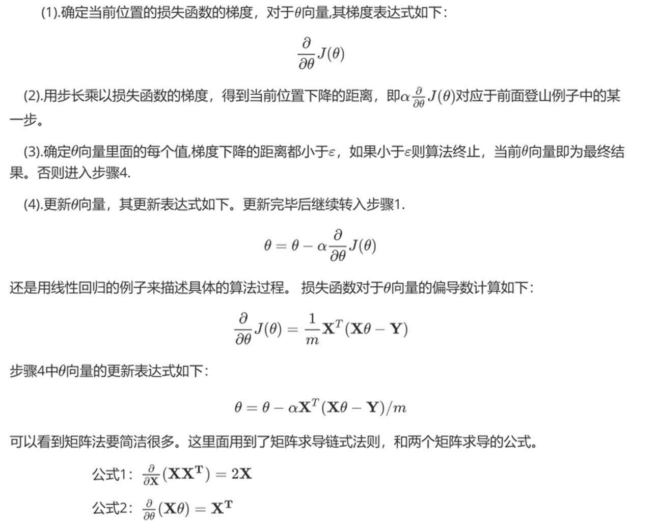
3.2 梯度下降法的矩阵方法描述
这一部分主要讲解梯度下降法的矩阵方式表述,相对于上面的代数法,要求有一定的矩阵分析的基础知识,尤其是矩阵求导的知识。
①. 先决条件:需要确定优化模型的假设函数和损失函数。对于线性回归,假设函数hθ(x1, x2,... xn) = θ0 + θ1x1 + ... + θnxn的矩阵表达方式为:hθ(x) = Xθ
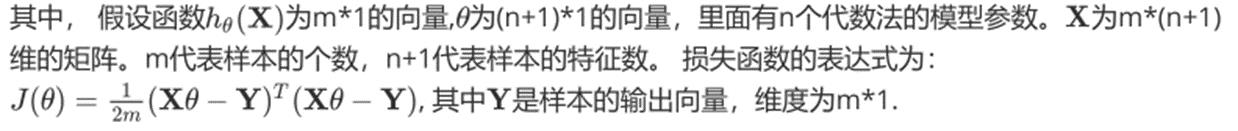
②. 算法相关参数初始化:θ向量可以初始化为默认值,或者调优后的值。算法终止距离ε,步长α和3.1比没有变化。
③. 算法过程:
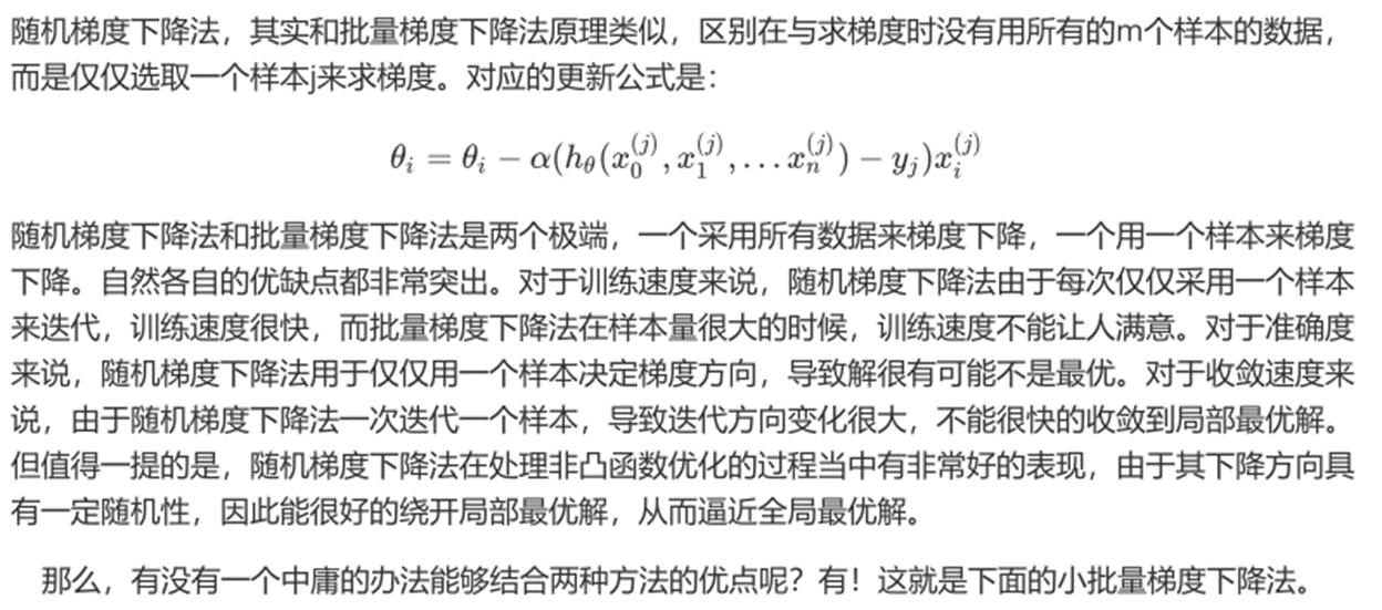
4. 梯度下降的种类
4.1 批量梯度下降法BGD

4.2 随机梯度下降法SGD
4.3 小批量梯度下降法MBGD


5. 梯度下降的算法调优
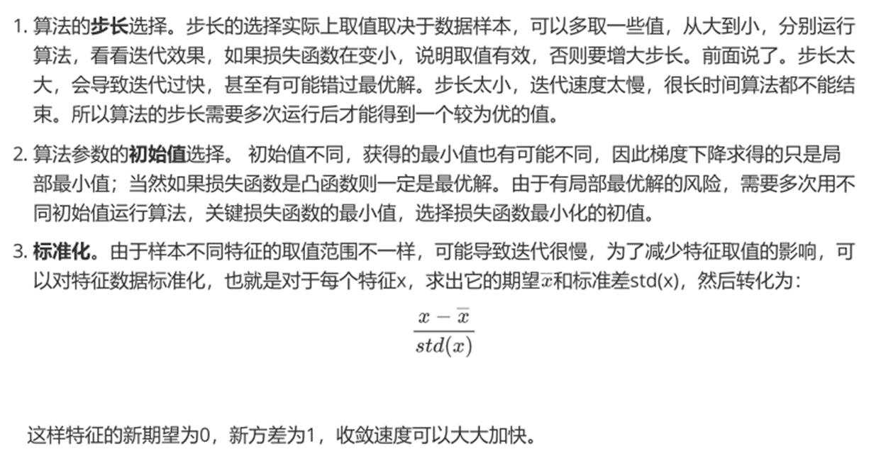
三、使用梯度下降求解逻辑回归
testSet数据集中一共有100个点,每个点包含两个数值型特征:X1和X2。因此可以将数据在一个二维平面上展示出来。我们可以将第一列数据(X1)看作x轴上的值,第二列数据(X2)看作y轴上的值。而最后一列数据即为分类标签。根据标签的不同,对这些点进行分类。
在此数据集上,我们将通过批量梯度下降法和随机梯度下降法找到最佳回归系数。
1. 使用BGD求解逻辑回归
批量梯度下降法的伪代码:
每个回归系数初始化为1
重复下面步骤直至收敛:
计算整个数据集的梯度
使用alpha*gradient更新回归系数的向量
返回回归系数
1.1 导入数据集
import pandas as pd
import numpy as np
import matplotlib.pyplot as plt
%matplotlib inline
dataSet = pd.read_table(\'testSet.txt\',header = None)
dataSet.columns =[\'X1\',\'X2\',\'labels\']
dataSet
可视化
plt.figure()
plt.scatter(dataSet[dataSet[\'labels\']==0][\'X1\'],dataSet[dataSet[\'labels\']==0]
[\'X2\'],c=\'red\')
plt.scatter(dataSet[dataSet[\'labels\']==1][\'X1\'],dataSet[dataSet[\'labels\']==1]
[\'X2\'],c=\'blue\')
plt.show()

1.2 定义辅助函数
Sigmoid函数
def sigmoid(inX):
    """
        函数功能:计算sigmoid函数值
        参数说明:
            inX:数值型数据
        返回:
            s:经过sigmoid函数计算后的函数值
    """
  s = 1/(1+np.exp(-inX))
  return s
标准化函数
def regularize(xMat):
    """
        函数功能:标准化(期望为0,方差为1)
        参数说明:
            xMat:特征矩阵
        返回:
            inMat:标准化之后的特征矩阵
    """
  inMat = xMat.copy()
  inMeans = np.mean(inMat,axis = 0)
  inVar = np.std(inMat,axis = 0)
  inMat = (inMat - inMeans)/inVar
  return inMat
1.3 BGD算法python实现
def BGD_LR(dataSet,alpha=0.001,maxCycles=500):
    """
        函数功能:使用BGD求解逻辑回归
        参数说明:
            dataSet:DF数据集
            alpha:步长
            maxCycles:最大迭代次数
        返回:
            weights:各特征权重值
    """
    xMat = np.mat(dataSet.iloc[:,:-1].values)
    yMat = np.mat(dataSet.iloc[:,-1].values).T
    xMat = regularize(xMat)
    m,n = xMat.shape
    weights = np.zeros((n,1))
    for i in range(maxCycles):
        grad = xMat.T*(xMat * weights-yMat)/m
        weights = weights -alpha*grad
    return weights
ws=BGD_LR(dataSet,alpha=0.01,maxCycles=500)
xMat = np.mat(dataSet.iloc[:, :-1].values)
yMat = np.mat(dataSet.iloc[:, -1].values).T
xMat = regularize(xMat)
(xMat * ws).A.flatten()
p = sigmoid(xMat * ws).A.flatten()
for i, j in enumerate(p):
  if j < 0.5:
    p[i] = 0
  else:
    p[i] = 1
train_error = (np.fabs(yMat.A.flatten() - p)).sum()
train_error_rate = train_error / yMat.shape[0]
train_error_rate
1.4 准确率计算函数
将上述过程封装为函数,方便后续调用
def logisticAcc(dataSet, method, alpha=0.01, maxCycles=500):
    """
        函数功能:计算准确率
        参数说明:
            dataSet:DF数据集
            method:计算权重函数
            alpha:步长
            maxCycles:最大迭代次数
        返回:
            trainAcc:模型预测准确率
    """
    weights = method(dataSet,alpha=alpha,maxCycles=maxCycles)
    p = sigmoid(xMat * ws).A.flatten()
    for i, j in enumerate(p):
        if j < 0.5:
            p[i] = 0
        else:
            p[i] = 1
    train_error = (np.fabs(yMat.A.flatten() - p)).sum()
    trainAcc = 1 - train_error / yMat.shape[0]
    return trainAcc
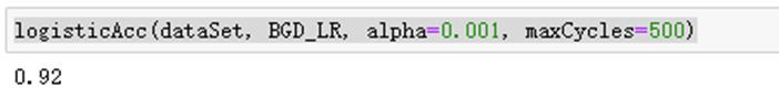
# 测试函数运行结果
logisticAcc(dataSet, BGD_LR, alpha=0.001, maxCycles=500)
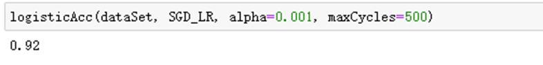
2. 使用SGD求解逻辑回归
随机梯度下降法的伪代码:
每个回归系数初始化为1
对数据集中每个样本:
计算该样本的梯度
使用alpha*gradient更新回归系数值
返回回归系数值
2.1 SGD算法python实现
def SGD_LR(dataSet,alpha=0.001,maxCycles=500):
    """
        函数功能:使用SGD求解逻辑回归
        参数说明:
            dataSet:DF数据集
            alpha:步长
            maxCycles:最大迭代次数
        返回:
            weights:各特征权重值
    """
    dataSet = dataSet.sample(maxCycles, replace=True)
    dataSet.index = range(dataSet.shape[0])
    xMat = np.mat(dataSet.iloc[:, :-1].values)
    yMat = np.mat(dataSet.iloc[:, -1].values).T
    xMat = regularize(xMat)
    m, n = xMat.shape
    weights = np.zeros((n,1))
    for i in range(m):
        grad = xMat[i].T * (xMat[i] * weights - yMat[i])
        weights = weights - alpha * grad
    return weights

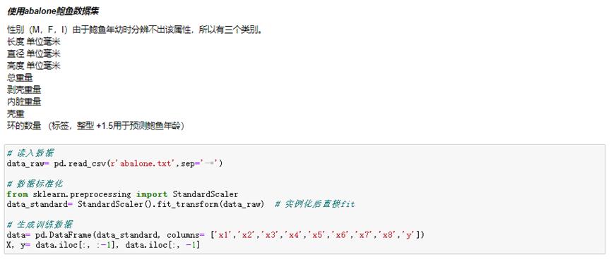
四、从疝气病症预测病马的死亡率
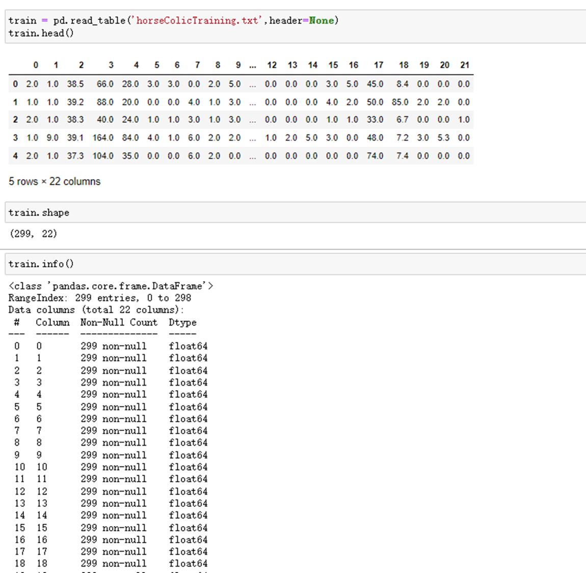
将使用Logistic回归来预测患疝气病的马的存活问题。原始数据集下载地址:http://archive.ics.uci.edu/ml/datasets/Horse+Colic
这里的数据包含了368个样本和28个特征。这种病不一定源自马的肠胃问题,其他问题也可能引发马疝病。该数据集中包含了医院检测 马疝病的一些指标,有的指标比较主观,有的指标难以测量,列如马的疼痛级别。另外需要说明的是,除了部分指标主观和难以测量外,该数据还存在一个问题,数据集中有30%的值是缺失的。下面将首先介绍如何处理数据集中的数据缺失问题,然后再利用Logistic回归和随机梯度上升算法来预测病马的生死。
1. 准备数据
数据中缺失值是一个非常棘手的问题,很多文献都致力于解决这个问题。那么,数据缺失究竟带来了什么问题?假设有100个样本和20个特征,这些数据都是机器收集回来的。若机器上的魔噩个传感器损坏导致一个特征无效时该怎么办?它们是否还可用》答案是肯定的。因为有时候数据相当昂贵,扔掉和重新获取都是不可取的,所以必须采用一些方法来解决这个问题。下面给出了一些可选的做法:
使用可用特征的均值来填补缺失值;
- 使用特殊值来填补缺失值,如-1;
- 忽略有缺失值的样本;
- 使用相似样本的均值填补缺失值;
- 使用另外的机器学习算法预测缺失值。
预处理数据做两件事:
- 如果测试集中一条数据的特征值已经缺失,那么我们选择实数0来替换所有缺失值,因为文本使用Logistic回归。因此这样做不会影响回归系数的值。sigmoid(0)=0.5,即它对结果的预测不具有任何倾向性。
- 如果测试集中一条数据的类别标签已经缺失,那么我们将类别数据丢弃,因为类别标签与特征不同,很难确定采用某个合适的值来替换。
原始的数据集经过处理,保存为两个文件:horseColicTest.txt和horseColicTraining.txt。
import pandas as pd
train = pd.read_table(\'horseColicTraining.txt\',header=None)
train.head()
train.shape
train.info()
test = pd.read_table(\'horseColicTest.txt\',header=None)
test.head()
test.shape
test.info()
读取数据,并查看数据基本情况。
2. logistic回归分类函数
得到训练集和测试集之后,我们可以利用前面的BGD_LR和SGC_LR得到训练集的weights。
这里需要定义一个分类函数,根据sigmoid函数返回的值来确定y是0还是1。
def classify(inX,weights):
    """
        函数功能:给定测试数据和权重,返回标签类别
        参数说明:
            inX:测试数据
            weights:特征权重
    """
  p = sigmoid(sum(inX * weights))
  if p < 0.5:
    return 0
  else:
    return 1
3. 构建logistic模型
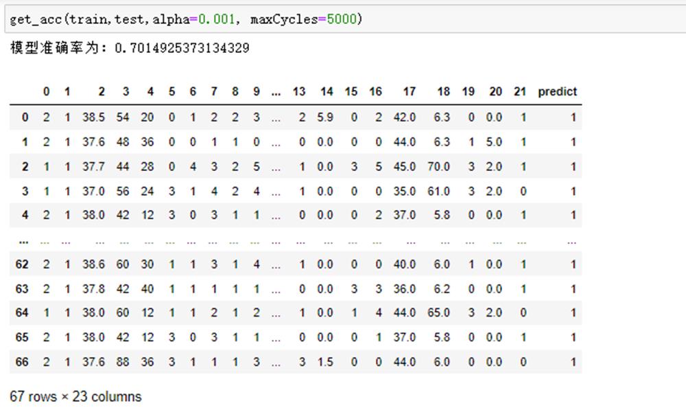
def get_acc(train,test,alpha=0.001, maxCycles=5000):
    """
        函数功能:logistic分类模型
        参数说明:
            train:测试集
            test:训练集
            alpha:步长
            maxCycles:最大迭代次数
        返回:
            retest:预测好标签的测试集
        """
    weights = SGD_LR(train,alpha=alpha,maxCycles=maxCycles)
    xMat = np.mat(test.iloc[:, :-1].values)
    xMat = regularize(xMat)
    result = []
    for inX in xMat:
        label = classify(inX,weights)
        result.append(label)
    retest=test.copy()
    retest[\'predict\']=result
    acc = (retest.iloc[:,-1]==retest.iloc[:,-2]).mean()
    print(f\'模型准确率为:acc\')
    return retest
测试函数运行结果:
运行10次查看结果:

从结果看出,模型预测的准确率基本维持在74%左右,原因有两点:①数据集本身有缺失值,我们处理之后对结果也会有影响;②逻辑回归这个算法本身也有上限。
五、 sklearn实现葡萄牙银行机构营销案例
案例背景:葡萄牙银行机构希望通过使用数据挖掘进行银行直接销售。所有的数据按日期排序(2008/5~2010/11)存储在bank-full.csv文件中。
分类目标位预测客户是否购买产品(定期存款)
特征为银行客户信息:

1. 导入数据集
#导入数据集,这里需要注意分隔符为分号“;”
bankSet = pd.read_csv(\'bank-full.csv\',sep=\';\')
bankSet.head()

#数据探索
bankSet.shape
bankSet.info()
bankSet.isnull().sum()#查看缺失值
2. 特征预处理
特征预处理这一块内容可参考菜菜讲的sklearn中的数据预处理和特征工程:https://www.bilibili.com/video/av36467376
- preprocessing.OrdinalEncoder:特征专用,能够将分类特征转换为分类数值
- preprocessing.LabelEncoder:(允许输入一维数据)标签专用,能够将分类转换为分类数值
- preprocessing.KBinsDiscretizer:这是将连续型变量划分为分类变量的类,能够将连续型变量排序后按顺序分箱后编码
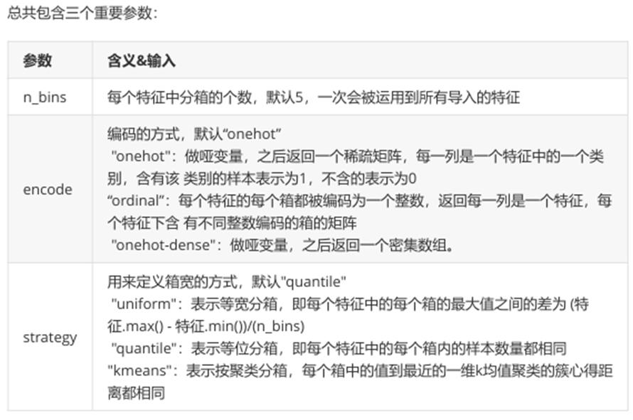
#将连续型变量分箱编码为分类变量
from sklearn.preprocessing import KBinsDiscretizer
#将age/duration/day字段编码为三分类变量
est1 = KBinsDiscretizer(n_bins=3, encode=\'ordinal\', strategy=\'kmeans\')
X1=bankSet.loc[:,[\'age\',\'duration\',\'day\']]
bankSet.loc[:,[\'age\',\'duration\',\'day\']]=est1.fit_transform(X1)

#将balance/campaign/pdays/previous字段编码为二分类变量
est2 = KBinsDiscretizer(n_bins=2, encode=\'ordinal\', strategy=\'kmeans\')
X2=bankSet.loc[:,[\'balance\',\'campaign\',\'pdays\',\'previous\']]
bankSet.loc[:,[\'balance\',\'campaign\',\'pdays\',\'previous\']]=est2.fit_transform(X2)

#查看编码后效果
bankSet.head()
bankSet[\'age\'].value_counts()
bankSet[\'balance\'].value_counts()

#将分类特征转换为分类数值
from sklearn.preprocessing import OrdinalEncoder
bankSet.iloc[:,:] = OrdinalEncoder().fit_transform(bankSet)
bankSet.head()
3. 切分训练集和测试集
from sklearn.model_selection import train_test_split
x_train,x_test,y_train,y_test = train_test_split(bankSet.iloc[:,:-1],bankSet.iloc[:,-1],test_size=0.25,random_state=0)
4. 构建逻辑回归分类函数
from sklearn.linear_model import LogisticRegression
#建模
classifier = LogisticRegression(random_state = 0)
classifier.fit(x_train,y_train)
#预测
y_pred = classifier.predict(x_test)
#计算模型准确率
from sklearn.metrics import accuracy_score
accuracy_score(y_test,y_pred)
六、 分类算法大比拼
1. 导入数据集
#导入数据
dataset = pd.read_csv(\'Social_Network_Ads.csv\')
dataset.head()
#探索数据
dataset.shape
dataset.info()
2. 数据预处理
#这里只需要处理性别这一个特征,所以用LabelEncoder,因为它允许输入一维数据
from sklearn.preprocessing import LabelEncoder
dataset.loc[:,\'Gender\']=LabelEncoder().fit_transform(dataset.loc[:,\'Gender\'])
3. 切分训练集和测试集
#提取出特征矩阵和标签
x = dataset.iloc[:,1:-1].values
y = dataset.iloc[:,-1].values
#切分训练集和测试集
from sklearn.model_selection import train_test_split
x_train,x_test,y_train,y_test = train_test_split(x,y
                        ,test_size=0.25
                        ,random_state=0)
#查看训练集
x_train[:10]
#数据标准化(StandardScaler作用:针对每一个特征维度去均值和方差归一化)
from sklearn.preprocessing import StandardScaler
sc = StandardScaler()
x_train = sc.fit_transform(x_train)
x_test = sc.fit_transform(x_test)
#查看标准化后的训练集
x_train[:10]
4. 各分类算法建模
4.1 logistic回归
#建模及预测
from sklearn.linear_model import LogisticRegression
logreg = LogisticRegression()
logreg.fit(x_train, y_train)
y_pred = logreg.predict(x_test)
acc_log = round(logreg.score(x_train, y_train) * 100, 2)
acc_log
4.2 KNN
from sklearn.neighbors import KNeighborsClassifier
knn = KNeighborsClassifier(n_neighbors = 3)
knn.fit(x_train, y_train)
y_pred = knn.predict(x_test)
acc_knn = round(knn.score(x_train, y_train) * 100, 2)
acc_knn
4.3 高斯朴素贝叶斯
from sklearn.naive_bayes import GaussianNB
gaussian = GaussianNB()
gaussian.fit(x_train, y_train)
y_pred = gaussian.predict(x_test)
acc_gaussian = round(gaussian.score(x_train, y_train) * 100, 2)
acc_gaussian
4.4 决策树
decision_tree = DecisionTreeClassifier()
decision_tree.fit(x_train, y_train)
y_pred = decision_tree.predict(x_test)
acc_decision_tree = round(decision_tree.score(x_train, y_train) * 100, 2)
acc_decision_tree
4.5 随机森林
from sklearn.ensemble import RandomForestClassifier
random_forest = RandomForestClassifier(n_estimators=100)
random_forest.fit(x_train, y_train)
y_pred = random_forest.predict(x_test)
random_forest.score(x_train, y_train)
acc_random_forest = round(random_forest.score(x_train, y_train) * 100, 2)
acc_random_forest
4.6 结果汇总
models = pd.DataFrame(
  \'Model\': [\'Logistic Regression\', \'KNN\',
       \'Naive Bayes\', \'Random Forest\',
       \'Decision Tree\'],
  \'Score\': [ acc_log,acc_knn, acc_gaussian,
       acc_random_forest,acc_decision_tree])
models.sort_values(by=\'Score\', ascending=False)
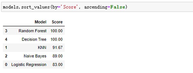
依次为随机森林-决策树-k-近邻算法-高斯朴素贝叶斯-逻辑回归
七、 算法总结
1. logistic优点
1.1 形式简单,模型的可解释性非常好。从特征的权重可以看到不同的特征第最后结果的影响,某个特征的权重值比较高,那么这个特征最后对结果的影响会比较大。
1.2 逻辑回归的对率函数是任意阶可导函数,数学性质号,易于优化。
1.3 逻辑回归不仅可以预测类别,还可以得到近似的概率预测。
1.4 模型效果不错。在工程上是可以接受的(最为baseline),如果特征工程做到好,效果不会太差,并且特征工程可以大家并行开发,大大加快开发的速度。
1.5 训练速度较快。分类的时候,计算量进京只和特征的数目相关。并且逻辑回归的分布式游湖sgd发展比较成熟,训练的速度可以通过堆机器进一步提高,这样我们可以在短时间内迭代好几个版本的模型。
1.6 方便输出结果调用。逻辑回归可以很方便的得到最后的分类结果,因为输出的是每个样本的概率分数,我们可以很容易的对这些概率分数进行cutoff,也就是划分阈值(大于某个阈值的是一类,小于某个阈值的是一类)。
2. logistic缺点
2.1 准确率并不是很高。因为形式非常的简单(非常类似线性模型),很难去拟合数据的真实分布。
2.2 很难处理数据不平衡的问题。比如:如果我们对于一个正负样本非常不平衡的问题比如正负样本比较10000:1。我们把所有样本都预测为正也能是损失函数的值比较小。但是作为一个分类器,它对正负样本的区分能力不会很好。
2.3 处理非线性数据较麻烦。逻辑回归在不引入其他方法的情况下,只能处理线性可分的数据。
2.4 逻辑回归本身无法筛选特征。有时候,我们会用gbdt来筛选特征,然后再上逻辑回归。
3. LR与SVM的关系
3.1 相同
① 都是有监督分类方法,判别模型(直接估计y=f(x)或p(y|x))
② 都是线性分类方法(指不用核函数的情况)
3.2 不同
① loss不同。LR是交叉熵,SVM是Hinge loss,最大话函数问题。
② LR决策考虑所有样本点,SVM决策仅仅取决于支持向量。
③ LR收数据分布影响,尤其是样本不均衡时影响大,要先做平衡,SVM不直接依赖于分布。
④ LR可以产生概率,SVM不能。
⑤ LR是经验风险最小化,需要另外加正则,SVM自带结构风险最小不需要加正则项。
⑥ LR每两个点之间都要做内积,而SVM只需要计算样本和支持向量的内积,计算量更小。
八、 案例分享
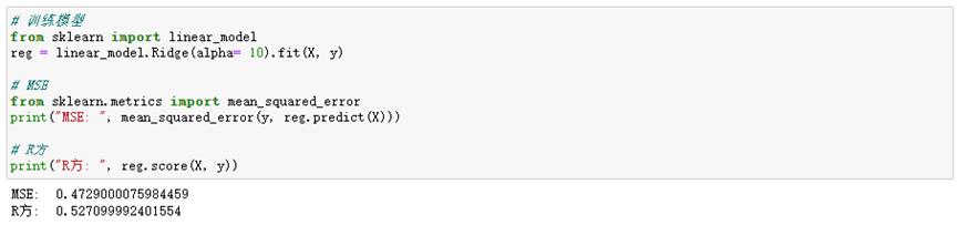
案例一 L1/L2正则化
1 岭回归手动实现(解析解)
导入数据库

岭回归函数定义


lam参数可以自由调整,目前往小调,theta会逐渐变大!
2 Sklearn中的岭回归
2.1 岭回归(L2正则)
一般用于模型调优处理。
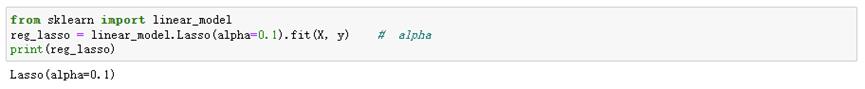
2.2 Lasso回归(L1正则)
一般用于变量选择。
2.3 弹性网络(L1+L2正则)

案例二 sklearn中的逻辑回归
1 Sklearn中的逻辑回归
导入库
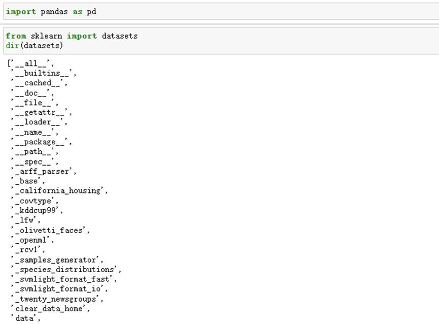
在sklearn的datasets中有多种数据集,其中fetch为在线数据集,load为本地数据集,make为模拟数据集。
\'fetch_california_housing\' 在线回归数据集
‘load_breast_cancer’ 本地二分类数据集
‘load_iris’ 本地多分类数据集
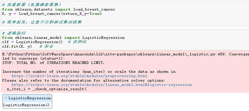
加载二分类的数据集并建模
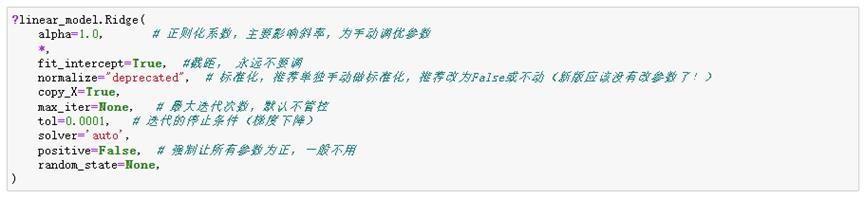
逻辑回归模型调优参数,标红色部分为一般调优参数,其他则根据需求进行调整。

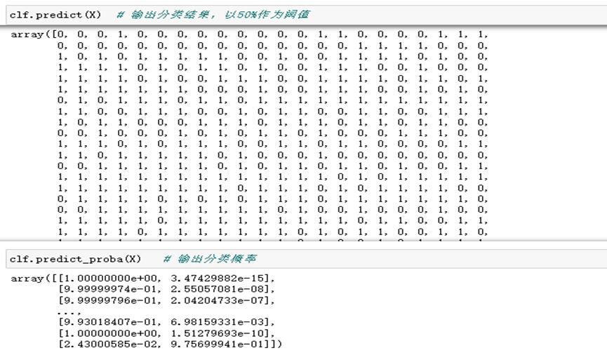
2 分类器评估
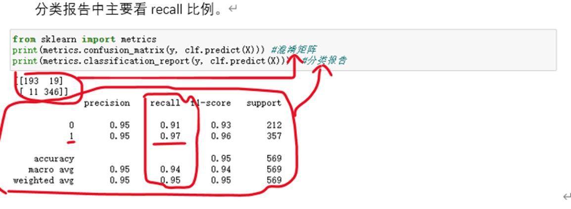
2.1 混淆矩阵和召回率
2.2 ROC曲线绘制

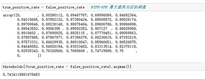
2.3 通过约登指数找最优阈值
案例三 Spark中的逻辑回归

1 Spark实现回归
1.1 线性回归
1.2 逻辑回归
数据集介绍

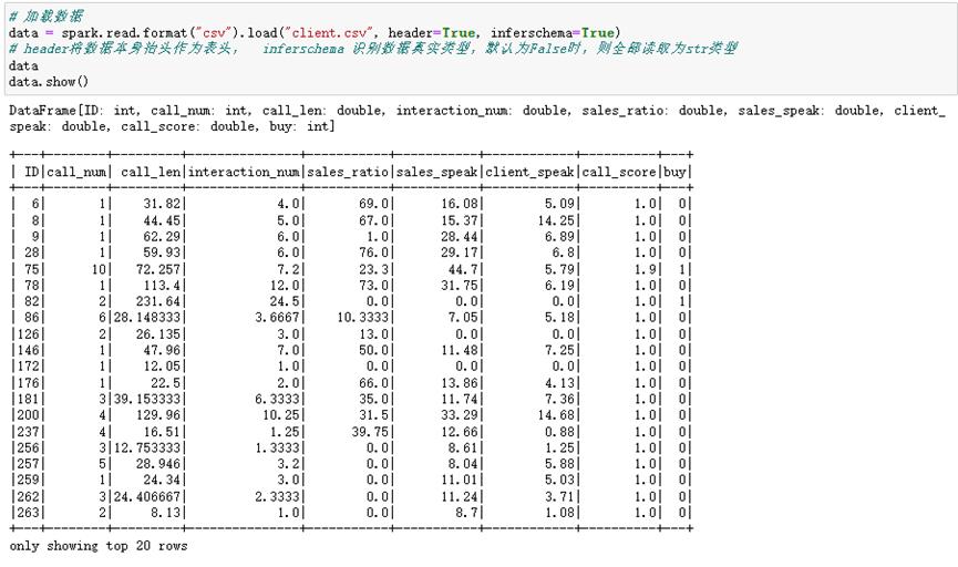
从数据上来看,count数据皆为10000,故没有缺失值。数据有正常的mean、std以及四分位点等信息,故没有异常符号等。

数据清洗,需要的时候可以使用。

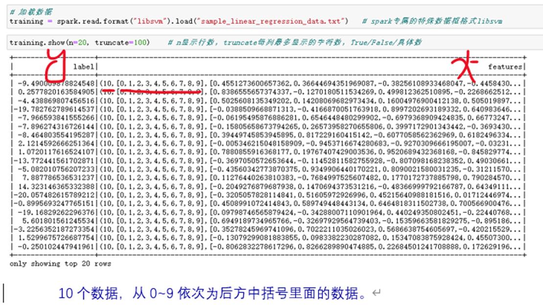
生成Spark专属特征数据集
首先需要挑出inputCols数据集,以下两种方式:
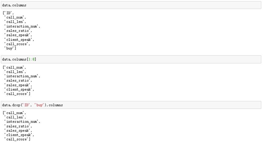
提供数据集,生成Spark专属数据集

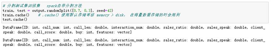
分割训练集和测试集
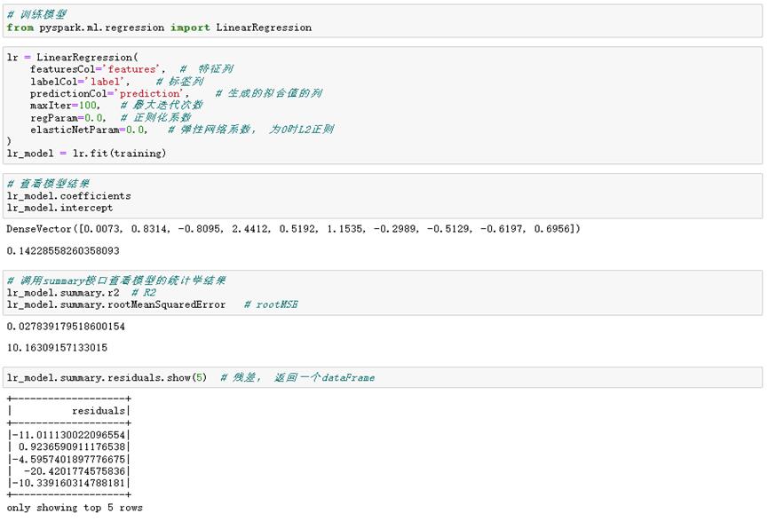
建模并训练模型
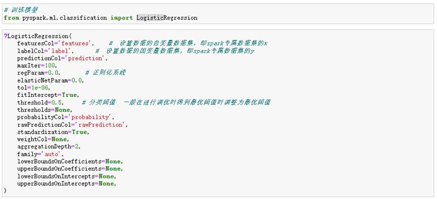
逻辑回归模型参数
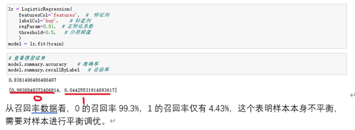
建模以及模型结果确认
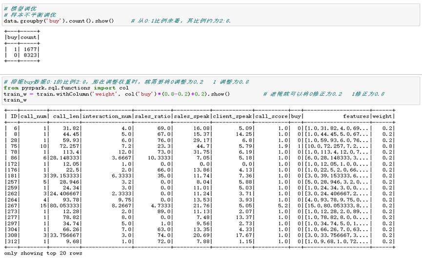
再次将该调优后的数据再次建模

调优后,从召回率数据看,0的召回率73.1%,1的召回率仅有58.1%,调优效果还是不错的。
预测

机器学习之逻辑回归(Logistic Regression)


-
"""逻辑回归中的Sigmoid函数"""
-
import numpy as np
-
import matplotlib.pyplot as plt
-
-
def sigmoid(t):
-
return 1/(1+np.exp(-t))
-
-
x=np.linspace(-10,10,500)
-
y=sigmoid(x)
-
-
plt.plot(x,y)
-
plt.show()
结果:


逻辑回归损失函数的梯度:


逻辑回归算法:
-
import numpy as np
-
from metrics import accuracy_score
-
-
class LogisticRegression:
-
-
def __init__(self):
-
"""初始化Logistic Regression模型"""
-
self.coef_ = None
-
self.intercept_ = None
-
self._theta = None
-
-
def _sigmoid(self,t):
-
return 1. / (1. + np.exp(-t))
-
-
def fit(self, X_train, y_train, eta=0.01, n_iters=1e4):
-
"""根据训练数据集X_train, y_train, 使用梯度下降法训练Linear Regression模型"""
-
assert X_train.shape[0] == y_train.shape[0],
-
"the size of X_train must be equal to the size of y_train"
-
-
-
-
def J(theta, X_b, y):
-
"""求损失函数"""
-
y_hat=self._sigmoid(X_b.dot(theta))
-
try:
-
return -np.sum(y*np.log(y_hat) + (1-y)*np.log(1-y_hat))/ len(y)
-
except:
-
return float(‘inf‘)
-
-
def dJ(theta, X_b, y):
-
"""求梯度"""
-
# res = np.empty(len(theta))
-
# res[0] = np.sum(X_b.dot(theta) - y)
-
# for i in range(1, len(theta)):
-
# res[i] = (X_b.dot(theta) - y).dot(X_b[:, i])
-
# return res * 2 / len(X_b)
-
return X_b.T.dot(self._sigmoid(X_b.dot(theta)) - y) / len(X_b)
-
-
def gradient_descent(X_b, y, initial_theta, eta, n_iters=1e4, epsilon=1e-8):
-
"""使用批量梯度下降法寻找theta"""
-
theta = initial_theta
-
cur_iter = 0
-
-
while cur_iter < n_iters:
-
gradient = dJ(theta, X_b, y)
-
last_theta = theta
-
theta = theta - eta * gradient
-
if (abs(J(theta, X_b, y) - J(last_theta, X_b, y)) < epsilon):
-
break
-
-
cur_iter += 1
-
-
return theta
-
-
X_b = np.hstack([np.ones((len(X_train), 1)), X_train])
-
initial_theta = np.zeros(X_b.shape[1])
-
self._theta = gradient_descent(X_b, y_train, initial_theta, eta, n_iters)
-
-
self.intercept_ = self._theta[0]
-
self.coef_ = self._theta[1:]
-
-
return self
-
-
def predict_proba(self, X_predict):
-
"""给定待预测数据集X_predict,返回表示X_predict的结果概率向量"""
-
assert self.intercept_ is not None and self.coef_ is not None,
-
"must fit before predict!"
-
assert X_predict.shape[1] == len(self.coef_),
-
"the feature number of X_predict must be equal to X_train"
-
-
X_b = np.hstack([np.ones((len(X_predict), 1)), X_predict])
-
return self._sigmoid(X_b.dot(self._theta))
-
-
def predict(self, X_predict):
-
"""给定待预测数据集X_predict,返回表示X_predict的结果向量"""
-
assert self.intercept_ is not None and self.coef_ is not None,
-
"must fit before predict!"
-
assert X_predict.shape[1] == len(self.coef_),
-
"the feature number of X_predict must be equal to X_train"
-
-
proba=self.predict_proba(X_predict)
-
return np.array(proba>=0.5,dtype=‘int‘)
-
-
def score(self, X_test, y_test):
-
"""根据测试数据集 X_test 和 y_test 确定当前模型的准确度"""
-
-
y_predict = self.predict(X_test)
-
return accuracy_score(y_test, y_predict)
-
-
def __repr__(self):
-
return "LogisticRegression()"
-
"""实现逻辑回归"""
-
import numpy as np
-
import matplotlib.pyplot as plt
-
from sklearn import datasets
-
-
iris=datasets.load_iris()
-
X=iris.data
-
y=iris.target
-
-
X=X[y<2,:2]
-
y=y[y<2]
-
-
plt.scatter(X[y==0,0],X[y==0,1],color=‘red‘)
-
plt.scatter(X[y==1,0],X[y==1,1],color=‘blue‘)
-
plt.show()
-
-
"""使用逻辑回归"""
-
from model_selection import train_test_split
-
from LogisticRegression import LogisticRegression
-
-
X_train,X_test,y_train,y_test=train_test_split(X,y,seed=666)
-
log_reg=LogisticRegression()
-
log_reg.fit(X_train,y_train)
-
print(log_reg.score(X_test,y_test))
-
print(log_reg.predict_proba(X_test))
结果:
-
E:pythonspaceKNN_functionvenvScriptspython.exe E:/pythonspace/KNN_function/try.py
-
1.0
-
[0.92972035 0.98664939 0.14852024 0.17601199 0.0369836 0.0186637
-
0.04936918 0.99669244 0.97993941 0.74524655 0.04473194 0.00339285
-
0.26131273 0.0369836 0.84192923 0.79892262 0.82890209 0.32358166
-
0.06535323 0.20735334]
-
-
Process finished with exit code 0
逻辑回归中的决策边界和添加多项式特征:
-
"""在逻辑回归中添加多项式特征"""
-
import numpy as np
-
import matplotlib.pyplot as plt
-
-
np.random.seed(666)
-
X=np.random.normal(0,1,size=(100,2))
-
y=np.array(X[:,0]**2+X[:,1]**2<1.5,dtype=‘int‘)
-
-
-
"""使用逻辑回归"""
-
from LogisticRegression import LogisticRegression
-
-
log_reg=LogisticRegression()
-
log_reg.fit(X,y)
-
-
"""绘制思路"""
-
def plot_decision_boundary(model,axis):
-
x0,x1 = np.meshgrid(
-
np.linspace(axis[0],axis[1],int((axis[1]-axis[0])*100)),
-
np.linspace(axis[2],axis[3],int((axis[3]-axis[2])*100))
-
)
-
X_new = np.c_[x0.ravel(),x1.ravel()]
-
y_predict = model.predict(X_new)
-
zz = y_predict.reshape(x0.shape)
-
from matplotlib.colors import ListedColormap
-
custom_cmap = ListedColormap([‘#EF9A9A‘,‘#FFF59D‘,‘#90CAF9‘])
-
plt.contourf(x0,x1,zz,linewidth=5,cmap=custom_cmap)
-
-
plot_decision_boundary(log_reg,axis=[-4,4,-4,4])
-
plt.scatter(X[y==0,0],X[y==0,1])
-
plt.scatter(X[y==1,0],X[y==1,1])
-
plt.show()
-
-
-
"""添加特征值,即升维"""
-
from sklearn.preprocessing import PolynomialFeatures
-
from sklearn.preprocessing import StandardScaler
-
from sklearn.pipeline import Pipeline
-
def PolynomialLogisticRegression(degree):
-
return Pipeline([
-
(‘Poly‘,PolynomialFeatures(degree=degree)),
-
(‘std_scaler‘,StandardScaler()),
-
(‘Logistic‘,LogisticRegression())
-
])
-
poly_log_reg = PolynomialLogisticRegression(degree=2)
-
poly_log_reg.fit(X,y)
-
plot_decision_boundary(poly_log_reg,axis=[-4,4,-4,4])
-
plt.scatter(X[y==0,0],X[y==0,1])
-
plt.scatter(X[y==1,0],X[y==1,1])
-
plt.show()
结果:


-
"""逻辑回归中使用正则化"""
-
import numpy as np
-
import matplotlib.pyplot as plt
-
from sklearn.model_selection import train_test_split
-
from sklearn.linear_model import LogisticRegression
-
from sklearn.preprocessing import StandardScaler
-
from sklearn.pipeline import Pipeline
-
from sklearn.preprocessing import PolynomialFeatures
-
-
np.random.seed(666)
-
X=np.random.normal(0,1,size=(200,2))
-
y=np.array(X[:,0]**2+X[:,1]<1.5,dtype=‘int‘)
-
for _ in range(20):
-
y[np.random.randint(200)] = 1
-
plt .scatter(X[y==0,0],X[y==0,1])
-
plt .scatter(X[y==1,0],X[y==1,1])
-
plt.show()
-
-
X_train,X_test,y_train,y_test=train_test_split(X,y)
-
log_reg=LogisticRegression()
-
log_reg.fit(X,y)
-
def plot_decision_boundary(model,axis):
-
x0,x1 = np.meshgrid(
-
np.linspace(axis[0],axis[1],int((axis[1]-axis[0])*100)),
-
np.linspace(axis[2],axis[3],int((axis[3]-axis[2])*100))
-
)
-
X_new = np.c_[x0.ravel(),x1.ravel()]
-
y_predict = model.predict(X_new)
-
zz = y_predict.reshape(x0.shape)
-
from matplotlib.colors import ListedColormap
-
custom_cmap = ListedColormap([‘#EF9A9A‘,‘#FFF59D‘,‘#90CAF9‘])
-
plt.contourf(x0,x1,zz,linewidth=5,cmap=custom_cmap)
-
-
def PolynomialLogisticRegression(degree,C=1.0,penalty=‘l2‘):
-
return Pipeline([
-
(‘Poly‘,PolynomialFeatures(degree=degree)),
-
(‘std_scaler‘,StandardScaler()),
-
(‘Logistic‘,LogisticRegression(C=C,penalty=penalty))
-
])
-
poly_log_reg = PolynomialLogisticRegression(degree=20,C=0.1,penalty=‘l1‘)
-
poly_log_reg.fit(X_train,y_train)
-
-
plot_decision_boundary(poly_log_reg,axis=[-4,4,-4,4])
-
plt.scatter(X[y==0,0],X[y==0,1])
-
plt.scatter(X[y==1,0],X[y==1,1])
-
plt.show()
结果

应用OVR和OVO使逻辑回归处理多分类问题
-
"""OVR和OVO"""
-
#为了数据可视化方便,我们只使用鸢尾花数据集的前两列特征
-
from sklearn import datasets
-
from sklearn.linear_model import LogisticRegression
-
from sklearn.model_selection import train_test_split
-
import matplotlib.pyplot as plt
-
import numpy as np
-
-
iris = datasets.load_iris()
-
X = iris[‘data‘][:,:2]
-
y = iris[‘target‘]
-
X_train,X_test,y_train,y_test=train_test_split(X,y,random_state=666)
-
-
-
#log_reg = LogisticRegression(multi_class=‘ovr‘) #传入multi_class参数可以指定使用ovr或ovo,默认ovr #由于只使用前两列特征,导致分类准确度较低
-
log_reg = LogisticRegression(multi_class=‘ovr‘,solver=‘newton-cg‘)
-
log_reg.fit(X_train,y_train)
-
log_reg.score(X_test,y_test)
-
def plot_decision_boundary(model,axis):
-
x0,x1 = np.meshgrid(
-
np.linspace(axis[0],axis[1],int((axis[1]-axis[0])*100)),
-
np.linspace(axis[2],axis[3],int((axis[3]-axis[2])*100))
-
)
-
X_new = np.c_[x0.ravel(),x1.ravel()]
-
y_predict = model.predict(X_new)
-
zz = y_predict.reshape(x0.shape)
-
from matplotlib.colors import ListedColormap
-
custom_cmap = ListedColormap([‘#EF9A9A‘,‘#FFF59D‘,‘#90CAF9‘])
-
plt.contourf(x0,x1,zz,linewidth=5,cmap=custom_cmap)
-
-
plot_decision_boundary(log_reg,axis=[4,8.5,1.5,4.5])
-
plt.scatter(X[y==0,0],X[y==0,1])
-
plt.scatter(X[y==1,0],X[y==1,1])
-
plt.scatter(X[y==2,0],X[y==2,1])
-
plt.show()
-
-
-
-
"""使用全部数据 OVR and OVO"""
-
from sklearn.multiclass import OneVsOneClassifier
-
from sklearn.multiclass import OneVsRestClassifier
-
-
from sklearn import datasets
-
from sklearn.linear_model import LogisticRegression
-
from sklearn.model_selection import train_test_split
-
iris = datasets.load_iris()
-
X = iris.data
-
y = iris.target
-
X_train,X_test,y_train,y_test=train_test_split(X,y,random_state=666)
-
-
ovr = OneVsRestClassifier(log_reg) #参数为二分类器
-
ovr.fit(X_train,y_train)
-
print(ovr.score(X_test,y_test))
-
ovo = OneVsOneClassifier(log_reg)
-
ovo.fit(X_train,y_train)
-
print(ovo.score(X_test,y_test))
结果:
-
E:pythonspaceKNN_functionvenvScriptspython.exe E:/pythonspace/KNN_function/try.py
-
E:pythonspaceKNN_functionvenvlibsite-packagesmatplotlibcontour.py:960: UserWarning: The following kwargs were not used by contour: ‘linewidth‘
-
s)
-
0.9736842105263158
-
1.0
-
-
Process finished with exit code 0

以上是关于0005.有监督学习之逻辑回归(Logistic回归)的主要内容,如果未能解决你的问题,请参考以下文章