ResNet网络

Posted 2023-05-05

参考技术A ResNet (Residual Neural Network，残差网络)由微软研究院何凯明等人提出的，通过在深度神经网络中加入残差单元（Residual Unit）使得训练深度比以前更加高效。ResNet在2015年的ILSVRC比赛中夺得冠军，ResNet的结构可以极快的加速超深神经网络的训练，模型准确率也有非常大的提升。

在ResNet之前，瑞士教授Schimidhuber提出了Highway Network，其原理与ResNet非常相似。通常认为神经网络的深度对其性能非常重要，但是网络越深训练越困难，Highway Network的目标就是解决极深的神经网络难以训练的问题。

Highway Network相当于修改了每一层激活函数，此前激活函数只是对输入做一次非线性变换y=H(x, Wh), 而Highway Network则允许保留一部分比例的原始输入x，即y=H(x, Wh)* T(x , Wt)+x*C(x, Wc)，其中T为变换系数，C为保留系数，论文中令C=1-T。这样前面一层的信息，有一定比例可以不经过矩阵乘法和非线性变换，直接传输到下一层，仿佛一条信息高速公路，因此得名Highway Network。

结果显示，B比A略好，这是因为A中的零填充确实没有残差学习。而C比B稍好，这是由于投影快捷连接引入了额外参数。但A、B、C之间的细微差异表明投影连接对于解决退化问题不是至关重要的，而不/少使用投影连接可以减少内存/时间复杂性和模型大小。而且无参数恒等快捷连接对于瓶颈架构（3层残差学习单元）尤为重要，因为瓶颈架构中层具有较小的输入输出，快捷连接是连接到两个高维端，此时恒等快捷连接无需参数，而使用投影的话则会显示时间和模型复杂度加倍。因此，恒等快捷连接可以为瓶颈设计得到更有效的模型。

最后，作者尝试了更深的1000层以上的神经网络，发现神经网络仍然能够较好的学习，但是其测试误差比100多层的残差网络要差，而训练误差则与100多层的残差网络相似，作者认为这可能是由于过拟合导致的，可通过加大正则化来解决这一问题。

在ResNet V1中，作者研究通过加入残差单元使得训练深度达到上百层的神经网络成为可能，解决了梯度消失/爆炸的问题。而在ResNet V2中作者进一步证明了恒等映射（Identity mapping）的重要性。同时作者还提出了一种新的残差单元（采用了预激活）使得训练变得更简单，同时还提高了模型的泛化能力。

在ResNet V2中，作者提出了不止在残差单元内部，而是在整个神经网络中都创建了‘直接’的计算传播路径。在ResNet V1中，残差学习单元的

上式同样表明了在一个mini-batch中不可能出现梯度消失的现象，因为上式求导的第二部分对于一个mini-batch来说，不可能所有样本其导数都为-1，因此，可能会出现权重很小的情况，但是不会出现梯度消失的情况。

通过研究这些不同的快捷连接，作者发现大部分快捷连接方式无法很好地收敛，其中很大部分是由于使用这些快捷连接后或多或少会出现梯度消失或者梯度爆炸的现象，最后结果显示恒等映射效果最好。

虽然恒等映射在这些方法中表写结果最好，仍需引起注意的是1×1的卷积捷径连接引入了更多的参数，本应该比恒等捷径连接具有更加强大的表达能力。事实上，shortcut-only gating 和1×1的卷积涵盖了恒等捷径连接的解空间(即，他们能够以恒等捷径连接的形式进行优化)。然而，它们的训练误差比恒等捷径连接的训练误差要高得多，这表明了这些模型退化问题的原因是优化问题，而不是表达能力的问题。

在上图b中，采用先加后BN再激活的方法，此时f(x)就包含了BN和ReLU。这样的结果比原始a要差。这主要是因为BN层改变了流经快捷连接的信号，阻碍了信息的传递。

在c中，ReLU在相加之前，此时f(x)=x，为恒等映射。此时残差单元中的F(x)输出经由ReLU后变为非负，然而一个“残差”函数的输出应该是(−∞,+∞) 的。造成的结果就是，前向传递的信号是单调递增的。这会影响表达能力，结果也变得更差了。

结果显示，只使用ReLU预激活（d）的结果与原始ResNet结果很接近，这个与ReLU层不与BN层连接使用，因此无法获得BN所带来的好处。而当BN和ReLU都使用在预激活上时（e），结果得到了可观的提升。

预激活的影响有两个方面：第一，由于f(x)也是恒等映射，相比于V1优化变得更加简单；第二，在预激活中使用BN能提高模型的正则化。

对于f(x)为恒等映射的好处：一方面若使用f= ReLU，如果信号是负的时候会造成一定的影响，无法传递有用的负信号，而当残差单元很多时，这个影响将会变得尤为突出；另一方面当f是一个恒等映射时，信号在两个单元间能够很直接的传递。

在ResNet V1中作者提出了残差学习单元，并从理论和实验上证明使用直连的shortcuts有助于解决深度达到上百层的神经网络的训练问题。而在ResNet V2中作者证明了在shortcuts中使用直接映射（即H(x) = h(x) + F(x)中h(x) = x）得到的效果最好。在ResNext中作者将bottleneck拆分成多个分支，提出了神经网络中的第三个维度（另外两个维度分别为depth，神经网络层数深度，width，宽度，channel数），命名为 Cardinality ，并在多个数据集中证明了将bottleneck拆分能够降低训练错误率和提高准确率。

ResNext的灵感来源于VGG/ResNet和Inception：（1）在VGG、ResNet中，作者使用了相同结构的卷积层进行了堆叠，构建了层数很深但是结构简单的神经网络；（2）而在Inception中，提出了一种叫做 split-transform-merge 的策略，将输入（采用1x1 卷积核）分裂为几个低维 embedding，再经过一系列特定卷积层的变换，最后连接在一起。

而在ResNet中，作者将原ResNet bottleneck中的一条path拆分为多个分支（multi branch），以此分支数量提出神经网络中的第三个重要维度——Cardinality。这一想法结合了VGG中的相同结构堆叠和Inception中的split-transform-merge策略，即如上图所示，每个bottleneck 拆分为多个分支进行堆叠，这些分支的结构相同（这里借鉴了VGG的思想），而具体到分支的结构时又采用了Inception的split-transform-merge策略。与Inception不同的是Inception的每个分支结构都是需要认为的设计，而在ResNext中每个分支结构都相同。最终每个bottleneck的输出就变成了：

这些所有的bottlenecks结构都遵循两个原则：

作者提出了 三种效果相同的ResNext的表示方法，如下图所示：

其中a,b 结构相似，只是在merge这一步的地方不同，而c则借鉴了AlexNet中分组卷积的思想，将输入和输出都分为多个组。

作者首先评估权衡了cardinality和width的关系。

接着，作者又评估了使用增加cardinality和depth/width来增加模型复杂度后的效果：

最后，作者还研究了shortcuts对于ResNext的重要性，在ResNet-50中，不使用shortcuts准确率下降了7%，而在ResNext-50中准确率也下降了4%，说明shortcuts对于残差网络来说确实是非常重要的。

简言之，增加cardinality比增加depth和width效果要好，同时，shortcuts对于模型的准确率也是至关重要的。

参考：
Deep Residual Learning for Image Recognition.
Aggregated Residual Transformations for Deep Neural Networks.
Identity Mappings in Deep Residual Networks.
ResNet论文翻译——中文版
Identity Mappings in Deep Residual Networks（译）
TensorFlow实现经典卷积网络. 黄文坚，唐源

Resnet 残差网络使用案例

Resnet 网络

Resnet是残差网络(Residual Network)的缩写,该系列网络广泛用于目标分类等领域以及作为计算机视觉任务主干经典神经网络的一部分，典型的网络有resnet50, resnet101等。Resnet网络的证明网络能够向更深（包含更多隐藏层）的方向发展。本篇是从国外的教程learnopencv 中的TensorFlow-Fully-Convolutional-Image-Classification而来，使用tensorflow2.1以上版本，文章中使用下载预训练的模型，改成了直接在本地中加载模型。

使用已经训练好的model

Resnet50_weights_tf_dim_ordering_tf_kernels_notop.h5 ，可以从https://storage.googleapis.com/tensorflow/keras-applications/resnet/ 直接下载
直接下载模型

效果

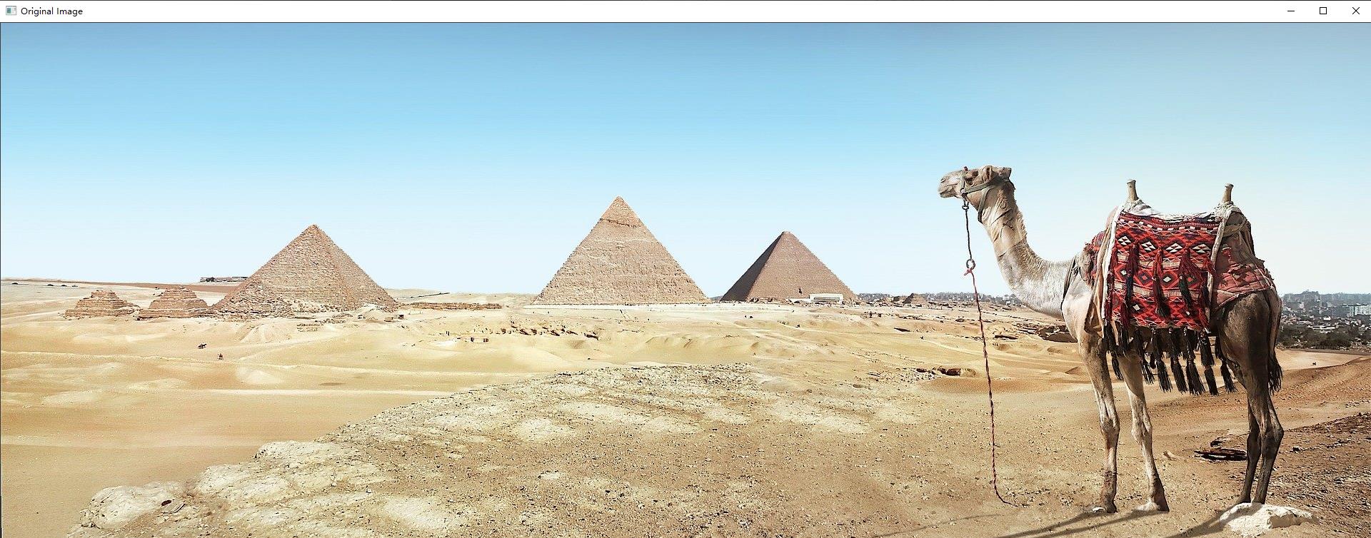
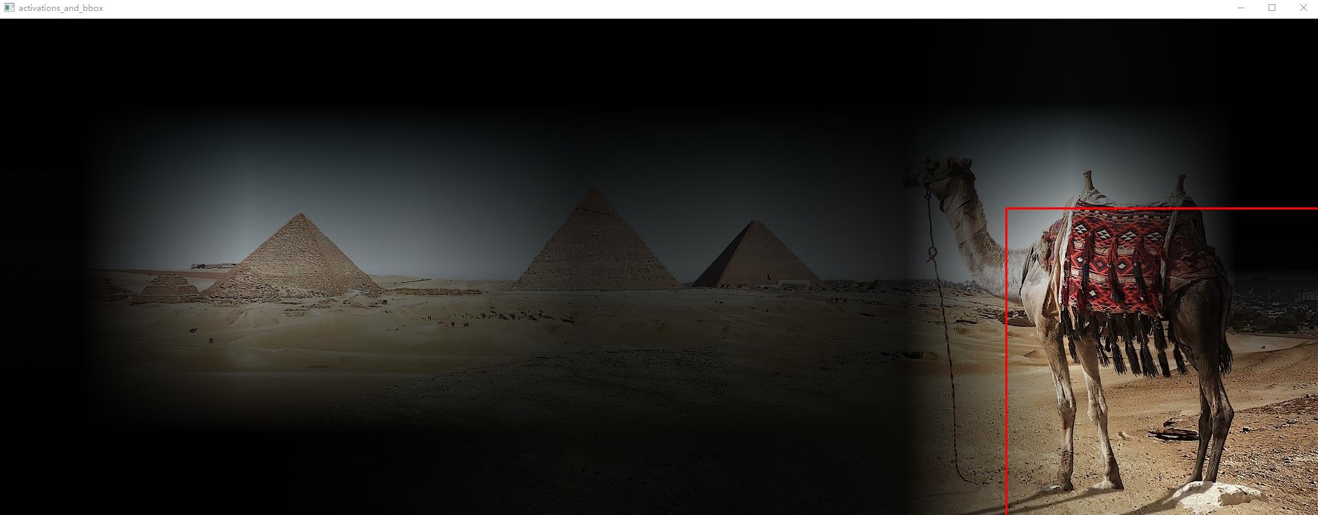
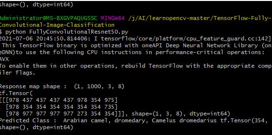
探测出一头阿拉伯单峰驼

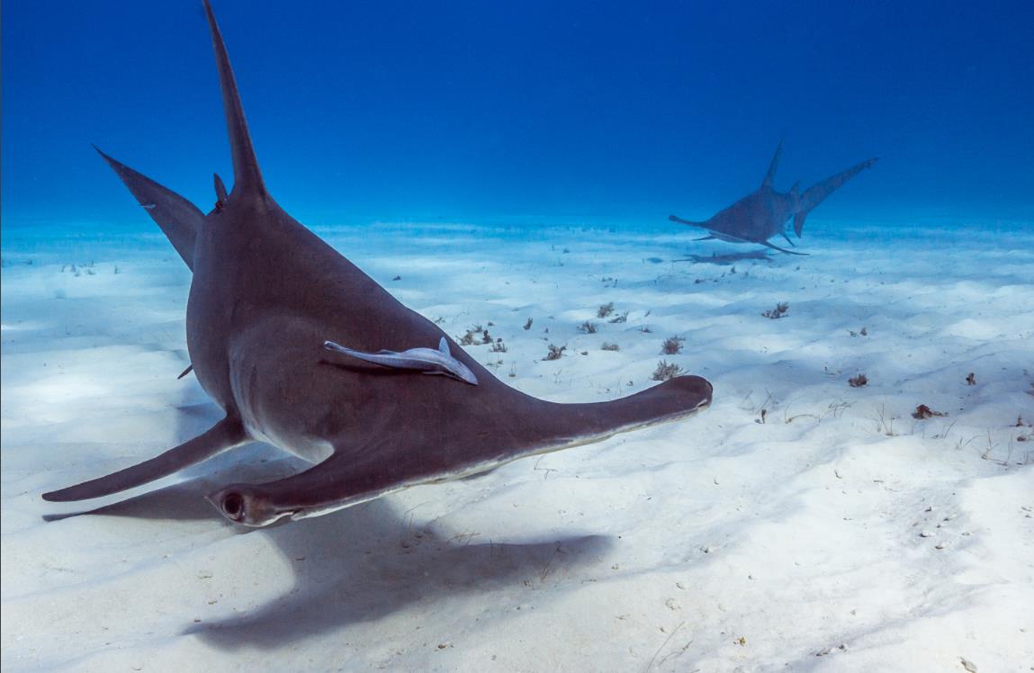
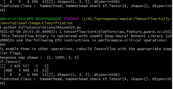
探测出是一头虎鲨

其他点

在卷积操作中，一般使用 padding=‘SAME’ 填充0，但有时不灵活，我们想自己去进行补零操作，此时可以使用tf.keras.layers.ZeroPadding2D

import cv2
import numpy as np
import tensorflow as tf
from tensorflow.keras import Input
from tensorflow.keras.applications import ResNet50
from tensorflow.keras.applications.resnet import preprocess_input
from tensorflow.keras.layers import (
    Activation,
    AveragePooling2D,
    BatchNormalization,
    Conv2D,
    MaxPooling2D,
    ZeroPadding2D,
)
from tensorflow.python.keras.engine import training
from tensorflow.python.keras.utils import data_utils

from utils import (
    BASE_WEIGHTS_PATH,
    WEIGHTS_HASHES,
    stack1,
)


#setting FC weights to the final convolutional layer
def set_conv_weights(model, feature_extractor):
    # get pre-trained ResNet50 FC weights
    dense_layer_weights = feature_extractor.layers[-1].get_weights()
    weights_list = [
        tf.reshape(
            dense_layer_weights[0], (1, 1, *dense_layer_weights[0].shape),
        ).numpy(),
        dense_layer_weights[1],
    ]
    model.get_layer(name="last_conv").set_weights(weights_list)


def fully_convolutional_resnet50(
    input_shape, num_classes=1000, pretrained_resnet=True, use_bias=True,
):
    # init input layer
    img_input = Input(shape=input_shape)

    # define basic model pipeline
    x = ZeroPadding2D(padding=((3, 3), (3, 3)), name="conv1_pad")(img_input)
    x = Conv2D(64, 7, strides=2, use_bias=use_bias, name="conv1_conv")(x)
    x = BatchNormalization(axis=3, epsilon=1.001e-5, name="conv1_bn")(x)
    x = Activation("relu", name="conv1_relu")(x)

    x = ZeroPadding2D(padding=((1, 1), (1, 1)), name="pool1_pad")(x)
    x = MaxPooling2D(3, strides=2, name="pool1_pool")(x)

    # the sequence of stacked residual blocks
    x = stack1(x, 64, 3, stride1=1, name="conv2")
    x = stack1(x, 128, 4, name="conv3")
    x = stack1(x, 256, 6, name="conv4")
    x = stack1(x, 512, 3, name="conv5")

    # add avg pooling layer after feature extraction layers
    x = AveragePooling2D(pool_size=7)(x)

    # add final convolutional layer
    conv_layer_final = Conv2D(
        filters=num_classes, kernel_size=1, use_bias=use_bias, name="last_conv",
    )(x)

    # configure fully convolutional ResNet50 model
    model = training.Model(img_input, x)

    # load model weights
    if pretrained_resnet:
        model_name = "resnet50"
        # configure full file name
        file_name = model_name + "_weights_tf_dim_ordering_tf_kernels_notop.h5"
        # get the file hash from TF WEIGHTS_HASHES
        #file_hash = WEIGHTS_HASHES[model_name][1]
        # weights_path = data_utils.get_file(
        #     file_name,
        #     BASE_WEIGHTS_PATH + file_name,
        #     cache_subdir="models",
        #     file_hash=file_hash,
        # )

        model.load_weights(file_name)

    # form final model
    model = training.Model(inputs=model.input, outputs=[conv_layer_final])

    if pretrained_resnet:
        # get model with the dense layer for further FC weights extraction
        resnet50_extractor = ResNet50(
            include_top=True, weights="imagenet", classes=num_classes,
        )
        # set ResNet50 FC-layer weights to final convolutional layer
        set_conv_weights(model=model, feature_extractor=resnet50_extractor)
    return model


if __name__ == "__main__":

    # read ImageNet class ids to a list of labels
    with open("imagenet_classes.txt") as f:
        labels = [line.strip() for line in f.readlines()]

    # read image
    original_image = cv2.imread("camel.jpg")

    # convert image to the RGB format
    image = cv2.cvtColor(original_image, cv2.COLOR_BGR2RGB)

    # pre-process image
    image = preprocess_input(image)

    # convert image to NCHW tf.tensor
    image = tf.expand_dims(image, 0)

    # load modified resnet50 model with pre-trained ImageNet weights
    model = fully_convolutional_resnet50(input_shape=(image.shape[-3:]))

    # Perform inference.
    # Instead of a 1×1000 vector, we will get a
    # 1×1000×n×m output ( i.e. a probability map
    # of size n × m for each 1000 class,
    # where n and m depend on the size of the image).
    preds = model.predict(image)
    preds = tf.transpose(preds, perm=[0, 3, 1, 2])
    preds = tf.nn.softmax(preds, axis=1)
    print("Response map shape : ", preds.shape)

    # find the class with the maximum score in the n × m output map
    pred = tf.math.reduce_max(preds, axis=1)
    class_idx = tf.math.argmax(preds, axis=1)
    print(class_idx)

    row_max = tf.math.reduce_max(pred, axis=1)
    row_idx = tf.math.argmax(pred, axis=1)

    col_idx = tf.math.argmax(row_max, axis=1)

    predicted_class = tf.gather_nd(
        class_idx, (0, tf.gather_nd(row_idx, (0, col_idx[0])), col_idx[0]),
    )

    # print top predicted class
    print("Predicted Class : ", labels[predicted_class], predicted_class)

    # find the n × m score map for the predicted class
    score_map = tf.expand_dims(preds[0, predicted_class, :, :], 0).numpy()
    score_map = score_map[0]

    # resize score map to the original image size
    score_map = cv2.resize(
        score_map, (original_image.shape[1], original_image.shape[0]),
    )

    # binarize score map
    _, score_map_for_contours = cv2.threshold(
        score_map, 0.65, 1, type=cv2.THRESH_BINARY,
    )
    score_map_for_contours = score_map_for_contours.astype(np.uint8).copy()

    # find the contour of the binary blob
    contours, _ = cv2.findContours(
        score_map_for_contours, mode=cv2.RETR_EXTERNAL, method=cv2.CHAIN_APPROX_SIMPLE,
    )

    # find bounding box around the object.
    rect = cv2.boundingRect(contours[0])

    # apply score map as a mask to original image
    score_map = score_map - np.min(score_map[:])
    score_map = score_map / np.max(score_map[:])

    score_map = cv2.cvtColor(score_map, cv2.COLOR_GRAY2BGR)
    masked_image = (original_image * score_map).astype(np.uint8)

    # display bounding box
    cv2.rectangle(
        masked_image, rect[:2], (rect[0] + rect[2], rect[1] + rect[3]), (0, 0, 255), 2,
    )

    # display images
    cv2.imshow("Original Image", original_image)
    cv2.imshow("scaled_score_map", score_map)
    cv2.imshow("activations_and_bbox", masked_image)
    cv2.waitKey(0)

这里是util.py

from tensorflow.keras.layers import (
    Activation,
    Add,
    BatchNormalization,
    Conv2D,
)

#https://github.com/tensorflow/tensorflow/blob/2b96f3662bd776e277f86997659e61046b56c315/tensorflow/python/keras/applications/resnet.py#L32
BASE_WEIGHTS_PATH = (
    "https://storage.googleapis.com/tensorflow/keras-applications/resnet/"
)
WEIGHTS_HASHES = {
    "resnet50": "4d473c1dd8becc155b73f8504c6f6626",
}


#https://github.com/tensorflow/tensorflow/blob/2b96f3662bd776e277f86997659e61046b56c315/tensorflow/python/keras/applications/resnet.py#L262
def stack1(x, filters, blocks, stride1=2, name=None):
    """
        A set of stacked residual blocks.
        Arguments:
          x: input tensor.
          filters: integer, filters of the bottleneck layer in a block.
          blocks: integer, blocks in the stacked blocks.
          stride1: default 2, stride of the first layer in the first block.
          name: string, stack label.
        Returns:
          Output tensor for the stacked blocks.
    """
    x = block1(x, filters, stride=stride1, name=name + "_block1")
    for i in range(2, blocks + 1):
        x = block1(x, filters, conv_shortcut=False, name=name + "_block" + str(i))
    return x


#https://github.com/tensorflow/tensorflow/blob/2b96f3662bd776e277f86997659e61046b56c315/tensorflow/python/keras/applications/resnet.py#L217
def block1(x, filters, kernel_size=3, stride=1, conv_shortcut=True, name=None):
    """
        A residual block.
        Arguments:
          x: input tensor.
          filters: integer, filters of the bottleneck layer.
          kernel_size: default 3, kernel size of the bottleneck layer.
          stride: default 1, stride of the first layer.
          conv_shortcut: default True, use convolution shortcut if True,
              otherwise identity shortcut.
          name: string, block label.
        Returns:
          Output tensor for the residual block.
    """
    # channels_last format
    bn_axis = 3

    if conv_shortcut:
        shortcut = Conv2D(4 * filters, 1, strides=stride, name=name + "_0_conv")(x)
        shortcut = BatchNormalization(
            axis=bn_axis, epsilon=1.001e-5, name=name + "_0_bn",
        )(shortcut)
    else:
        shortcut = x

    x = Conv2D(filters, 1, strides=stride, name=name + "_1_conv")(x)
    x = BatchNormalization(axis=bn_axis, epsilon=1.001e-5, name=name + "_1_bn")(x)
    x = Activation("relu", name=name + "_1_relu")(x)

    x = Conv2D(filters, kernel_size, padding="SAME", name=name + "_2_conv")(x)
    x = BatchNormalization(axis=bn_axis, epsilon=1.001e-5, name=name + "_2_bn")(x)
    x = Activation("relu", name=name + "_2_relu")(x)

    x = Conv2D(4 * filters, 1, name=name + "_3_conv")(x)
    x = BatchNormalization(axis=bn_axis, epsilon=1.001e-5, name=name + "_3_bn")(x)

    x = Add(name=name + "_add")([shortcut, x])
    x = Activation("relu", name=name + "_out")(x)
    return x

代码和图片

所有代码和图片以及模型