阅读A Comprehensive Survey on Distributed Training of Graph Neural Networks——翻译

Posted 2023-01-24 小锋学长生活大爆炸

Abstract

        Graph neural networks (GNNs) have been demonstrated to be a powerful algorithmic model in broad application fields for their effectiveness in learning over graphs. To scale GNN training up for large-scale and ever-growing graphs, the most promising solution is distributed training which distributes the workload of training across multiple computing nodes. However, the workflows, computational patterns, communication patterns, and optimization techniques of distributed GNN training remain preliminarily understood. In this paper, we provide a comprehensive survey of distributed GNN training by investigating various optimization techniques used in distributed GNN training. First, distributed GNN training is classified into several categories according to their workflows. In addition, their computational patterns and communication patterns, as well as the optimization techniques proposed by recent work are introduced. Second, the software frameworks and hardware platforms of distributed GNN training are also introduced for a deeper understanding. Third, distributed GNN training is compared with distributed training of deep neural networks, emphasizing the uniqueness of distributed GNN training. Finally, interesting issues and opportunities in this field are discussed.

        图形神经网络（GNN）在广泛的应用领域中被证明是一种强大的算法模型，因为其在图形学习中的有效性。为了将GNN训练扩展到大规模和不断增长的图形，最有希望的解决方案是分布式训练，它将训练的工作量分布在多个计算节点上。然而，分布式GNN训练的工作流程、计算模式、通信模式和优化技术仍有初步了解。在本文中，我们通过研究分布式GNN训练中使用的各种优化技术，对分布式GNN训练进行了全面的调查。首先，分布式GNN训练根据其工作流程分为几个类别。此外，还介绍了它们的计算模式和通信模式，以及最近工作提出的优化技术。其次，还介绍了分布式GNN训练的软件框架和硬件平台，以加深理解。第三，将分布式GNN训练与深度神经网络的分布式训练进行了比较，强调了分布式GNN训练的独特性。最后，讨论了该领域的有趣问题和机遇。

Index Terms

        Graph learning, graph neural network, distributed training, workflow, computational pattern, communication pattern, optimization technique, software framework.

        图形学习、图形神经网络、分布式训练、工作流、计算模式、通信模式、优化技术、软件框架。

INTRODUCTION

        GRAPH is a well-known data structure widely used in many critical application fields due to its powerful representation capability of data, especially in expressing the associations between objects [1], [2]. Many real-world data can be naturally represented as graphs which consist of a set of vertices and edges. Take social networks as an example [3], [4], the vertices in the graph represent people and the edges represent interactions between people on Facebook [5]. An illustration of graphs for social networks is illustrated in Fig. 1 (a), where the circles represent the vertices, and the arrows represent the edges. Another well-known example is knowledge graphs [6], [7], in which the vertices represent entities while the edges represent relations between the entities [8].

        GRAPH是一种众所周知的数据结构，由于其强大的数据表示能力，特别是在表达对象之间的关联[1]、[2]时，被广泛应用于许多关键应用领域。许多真实世界的数据可以自然地表示为由一组顶点和边组成的图形。以社交网络为例[3]，[4]，图中的顶点表示人，边表示Facebook上人与人之间的交互[5]。图1（a）说明了社交网络的图表，其中圆圈表示顶点，箭头表示边缘。另一个众所周知的例子是知识图[6]，[7]，其中顶点表示实体，而边表示实体之间的关系[8]。

        Graph neural networks (GNNs) demonstrate superior performance compared to other algorithmic models in learning over graphs [9]–[11]. Deep neural networks (DNNs) have been widely used to analyze Euclidean data such as images [12]. However, they have been challenged by graph data from the non-Euclidean domain due to the arbitrary size and complex topological structure of graphs [13]. Besides, a major weakness of deep learning paradigms identified by industry is that they cannot effectively carry out causal reasoning, which greatly reduces the cognitive ability of intelligent systems [14]. To this end, GNNs have emerged as the premier paradigm for graph learning and endowed intelligent systems with cognitive ability. An illustration for GNNs is shown in Fig. 1 (b). After getting graph data as input, GNNs use forward propagation and backward propagation to update the model parameters. Then the trained model can be applied to graph tasks, including vertex prediction [15] (predicting the properties of specific vertices), link prediction [16] (predicting the existence of an edge between two vertices), and graph prediction [17] (predicting the properties of the whole graph), as shown in Fig. 1 (c).

        与其他算法模型相比，图形神经网络（GNN）在图形学习方面表现出了优异的性能[9]-[11]。深度神经网络（DNN）已广泛用于分析图像等欧几里得数据[12]。然而，由于图的任意大小和复杂拓扑结构，它们受到了来自非欧几里得域的图数据的挑战[13]。此外，工业界发现的深度学习范式的一个主要弱点是它们不能有效地进行因果推理，这大大降低了智能系统的认知能力[14]。为此，GNN已成为图形学习的首要范式，并赋予智能系统认知能力。GNN的图示如图1（b）所示。在获得图形数据作为输入后，GNN使用正向传播和反向传播来更新模型参数。然后，训练后的模型可以应用于图形任务，包括顶点预测[15]（预测特定顶点的属性）、链接预测[16]（预测两个顶点之间的边的存在）和图形预测[17]（预测整个图形的属性），如图1（c）所示。

         Thanks to the superiority of GNNs, they have been widely used in various real-world applications in many critical fields. These real-world applications include knowledge inference [18], natural language processing [19], [20], machine translation [21], recommendation systems [22]–[24], visual reasoning [25], chip design [26]–[28], traffic prediction [29]– [31], ride-hailing demand forecasting [32], spam review detection [33], molecule property prediction [34], and so forth. GNNs enhance the machine intelligence when processing a broad range of real-world applications, such as giving>50% accuracy improvement for real-time ETAs in Google Maps [29], generating >40% higher-quality recommendations in Pinterest [22], achieving >10% improvement of ride-hailing demand forecasting in Didi [32], improving >66.90% of recall at 90% precision for spam review detection in Alibaba [33].

        由于GNN的优越性，它们已广泛应用于许多关键领域的各种现实应用中。这些实际应用包括知识推理[18]、自然语言处理[19]、[20]、机器翻译[21]、推荐系统[22]–[24]、视觉推理[25]、芯片设计[26]–[28]、交通预测[29]–[31]、叫车需求预测[32]、垃圾邮件审查检测[33]、分子属性预测[34]等。GNN在处理广泛的现实世界应用时增强了机器智能，例如，在谷歌地图中实时ETA的准确度提高了50%以上[29]，在Pinterest中生成了40%以上的高质量推荐[22]，在滴滴中实现了约车需求预测提高了10%以上[32]，阿里巴巴垃圾邮件审查检测的召回率提高了>66.90%，准确率为90%[33]。

        However, both industry and academia are still eagerly expecting the acceleration of GNN training for the following reasons [35]–[38]:

        然而，工业界和学术界仍热切期待GNN训练的加速，原因如下[35]–[38]：

        1. The scale of graph data is rapidly expanding, consuming a great deal of time for GNN training. With the explosion of information on the Internet, new graph data are constantly being generated and changed, such as the establishment and demise of interpersonal relationships in social communication and the changes in people's preferences for goods in online shopping. The scales of vertices and edges in graphs are approaching or even outnumbering the order of billions and trillions, respectively [39]–[42]. The growth rate of graph scales is also astonishing. For example, the number of vertices (i.e., users) in Facebook's social network is growing at a rate of 17% per year [43]. Consequently, GNN training time dramatically increases due to the ever-growing scale of graph data.

        1. 图形数据的规模正在迅速扩大，为GNN训练消耗了大量时间。随着互联网上信息的爆炸，新的图表数据不断产生和变化，例如社会交往中人际关系的建立和消亡，以及人们在网上购物中对商品偏好的变化。图中顶点和边的比例分别接近或超过数十亿和万亿量级[39]–[42]。图表规模的增长速度也惊人。例如，Facebook社交网络中的顶点（即用户）数量以每年17%的速度增长[43]。因此，由于图形数据的规模不断增长，GNN训练时间显著增加。

        2. Swift development and deployment of novel GNN models involves repeated training, in which a large amount of training time is inevitable. Much experimental work is required to develop a highly-accurate GNN model since repeated training is needed [9]–[11]. Moreover, expanding the usage of GNN models to new application fields also requires much time to train the model with real-life data. Such a sizeable computational burden calls for faster methods of training.

        2. 快速开发和部署新型GNN模型涉及重复训练，其中大量的训练时间是不可避免的。由于需要重复训练[9]-[11]，因此开发高精度GNN模型需要大量实验工作。此外，将GNN模型的使用扩展到新的应用领域也需要大量时间来使用真实数据训练模型。如此庞大的计算负担需要更快的训练方法。

        Distributed training is a popular solution to speed up GNN training [35]–[38], [40], [44]–[58]. It tries to accelerate the entire computing process by adding more computing resources, or "nodes", to the computing system with parallel execution strategies, as shown in Fig. 1 (d). NeuGraph [44], proposed in 2019, is the first published work of distributed GNN training. Since then, there has been a steady stream of attempts to improve the efficiency of distributed GNN training in recent years with significantly varied optimization techniques, including workload partitioning [44]–[47], transmission planning [37], [44]–[46], caching strategy [35], [51], [52], etc.

        分布式训练是加快GNN训练的流行解决方案[35]–[38]，[40]，[44]–[58]。它试图通过向具有并行执行策略的计算系统添加更多计算资源或“节点”来加速整个计算过程，如图1（d）所示。2019年提出的NeuGraph[44]是分布式GNN训练的第一个已发表的工作。从那时起，近年来有大量尝试通过显著不同的优化技术来提高分布式GNN训练的效率，包括工作负载划分[44]–[47]、传输规划[37]、[44]–[56]、缓存策略[35]、[51]、[52]等。

NeuGraph[44]是分布式GNN训练的第一个已发表的工作

        Despite the aforementioned efforts, there is still a dearth of review of distributed GNN training. The need for management and cooperation among multiple computing nodes leads to a different workflow, resulting in complex computational and communication patterns, and making it a challenge to optimize distributed GNN training. However, regardless of plenty of efforts on this aspect have been or are being made, there are hardly any surveys on these challenges and solutions. Current surveys mainly focus on GNN models and hardware accelerators [9]–[11], [59]–[62], but they are not intended to provide a careful taxonomy and a general overview of distributed training of GNNs, especially from the perspective of the workflows, computational patterns, communication patterns, and optimization techniques.

        尽管作出了上述努力，但仍缺乏对分布式GNN训练的审查。对多个计算节点之间的管理和合作的需求导致了不同的工作流，导致了复杂的计算和通信模式，并使优化分布式GNN训练成为一个挑战。然而，尽管在这方面已经或正在作出大量努力，但几乎没有任何关于这些挑战和解决方案的调查。当前的调查主要集中于GNN模型和硬件加速器[9]-[11]，[59]–[62]，但它们并非旨在提供GNN分布式训练的详细分类和一般概述，尤其是从工作流、计算模式、通信模式和优化技术的角度。

GNN模型和硬件加速器[9]-[11]，[59]–[62]

        This paper presents a comprehensive review of distributed training of GNNs by investigating its various optimization techniques. First, we summarize distributed GNN training into several categories according to their workflows. In addition, we introduce their computational patterns, communication patterns, and various optimization techniques proposed in recent works to facilitate scholars to quickly understand the principle of recent optimization techniques and the current research status. Second, we introduce the prevalent software frameworks and hardware platforms for distributed GNN training and their respective characteristics. Third, we emphasize the uniqueness of distributed GNN training by comparing it with distributed DNN training. Finally, we discuss interesting issues and opportunities in this field.

        本文通过研究GNN的各种优化技术，全面回顾了GNN的分布式训练。首先，我们根据工作流程将分布式GNN训练归纳为几个类别。此外，我们还介绍了它们的计算模式、通信模式以及最近工作中提出的各种优化技术，以帮助学者快速了解最近优化技术的原理和当前的研究现状。其次，我们介绍了用于分布式GNN训练的流行软件框架和硬件平台及其各自的特点。第三，通过与分布式DNN训练的比较，我们强调了分布式GNN训练的独特性。最后，我们讨论了这个领域的有趣问题和机遇。

        Our main goals are as follows:

        我们的主要目标如下：

        • Introducing the basic concepts of distributed GNN training.

        • 介绍分布式GNN训练的基本概念。

        • Analyzing the workflows, computational patterns, and communication patterns of distributed GNN training and summarizing the optimization techniques.

        • 分析分布式GNN训练的工作流程、计算模式和通信模式，总结优化技术。

        • Highlighting the differences between distributed GNN training and distributed DNN training.

        • 强调分布式GNN训练和分布式DNN训练之间的差异。

        • Discussing interesting issues and opportunities in the field of distributed GNN training.

        • 讨论分布式GNN训练领域的有趣问题和机会。

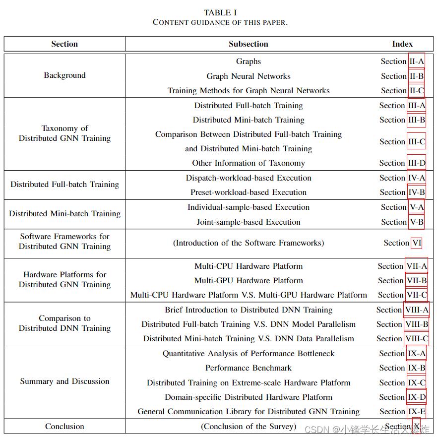
        The rest of this paper is described in accordance with these goals. Its organization is shown in Table I and summarized as follows:

        本文的其余部分将根据这些目标进行描述。其组织结构见表一，总结如下：

        • Section II introduces the basic concepts of graphs and GNNs as well as two training methods of GNNs: fullbatch training and mini-batch training.

        • 第二节介绍了图形和GNN的基本概念以及GNN的两种训练方法：全批量训练和小批量训练。

        • Section III introduces the taxonomy of distributed GNN training and makes a comparison between them.

        • 第三节介绍了分布式GNN训练的分类，并对其进行了比较。

        • Section IV introduces distributed full-batch training of GNNs and further categorizes it into two types, of which the workflows, computational patterns, communication patterns, and optimization techniques are introduced in detail.

        • 第四节介绍了GNN的分布式全批量训练，并将其进一步分类为两种类型，其中详细介绍了工作流、计算模式、通信模式和优化技术。

        • Section V introduces distributed mini-batch training and classifies it into two types. We also present the workflow, computational pattern, communication pattern, and optimization techniques for each type.

        • 第五节介绍了分布式小批量培训，并将其分为两种类型。我们还介绍了每种类型的工作流、计算模式、通信模式和优化技术。

        • Section VI introduces software frameworks currently supporting distributed GNN training and describes their characteristics.

        • 第六节介绍了目前支持分布式GNN训练的软件框架，并描述了其特点。

        • Section VII introduces hardware platforms for distributed GNN training.

        • 第七节介绍了分布式GNN培训的硬件平台。

        • Section VIII highlights the uniqueness of distributed GNN training by comparing it with distributed DNN training.

        • 第八节通过将分布式GNN训练与分布式DNN训练进行比较，强调了分布式GNN培训的独特性。

        • Section IX summarizes the distributed full-batch training and distributed mini-batch training, and discusses several interesting issues and opportunities in this field.

        • 第九节总结了分布式全批量训练和分布式小批量训练，并讨论了该领域的几个有趣问题和机会。

        • Section X is the conclusion of this paper.

        • 第十节是本文的结论。

 BACKGROUND

        This section provides some background concepts of graphs as well as GNNs, and introduces the two training methods applied in GNN training: full-batch and mini-batch.

        本节提供了图形和GNN的一些背景概念，并介绍了GNN训练中应用的两种训练方法：全批和小批。

A. Graphs

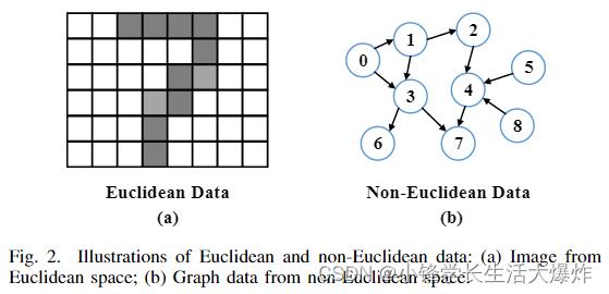
        A graph is a type of data structure consisting of vertices and edges. Its flexible structure can effectively express the relationship among a set of objects with arbitrary size and undetermined structure, which is called non-Euclidean data. As shown in Fig. 2 (a) and (b), the form of non-Euclidean data is not as highly structured as Euclidean data. However, by using vertices to represent the objects and edges to represent relationships among the objects, graphs can effectively represent non-Euclidean data, such as social networks and knowledge graphs.

        图是一种由顶点和边组成的数据结构。其灵活的结构可以有效地表达一组具有任意大小和不确定结构的对象之间的关系，称为非欧几里得数据。如图2（a）和（b）所示，非欧几里得数据的形式不像欧几里得数据那样高度结构化。然而，通过使用顶点来表示对象，使用边来表示对象之间的关系，图可以有效地表示非欧几里得数据，例如社交网络和知识图。

        There are mainly three taxonomies of graphs:

        图形主要有三种分类法：

        Directed/Undirected Graphs: Every edge in a directed graph has a fixed direction, indicating that the connection is only from a source vertex to a destination vertex. However, in an undirected graph, the connection represented by an edge is bi-directional between the two vertices. An undirected graph can be transformed into a directed one, in which two edges in the opposite direction represent an undirected edge in the original graph.

        有向/无向图：有向图中的每条边都有一个固定的方向，表示连接仅从源顶点到目标顶点。然而，在无向图中，由边表示的连接在两个顶点之间是双向的。一个无向图可以转化为一个有向图，其中两条相反方向的边表示原始图中的一条无向边。

        Homogeneous/Heterogeneous Graphs: Homogeneous graphs contain a single type of vertex and edge, while heterogeneous graphs contain multiple types of vertices and multiple types of edges. Thus, heterogeneous graphs are more powerful in expressing the relationships between different objects.

        同构/异构图：同构图包含单一类型的顶点和边，而异构图包含多种类型的顶点以及多种类型的边。因此，异构图在表达不同对象之间的关系方面更为强大。

        Static/Dynamic Graphs: The structure and the feature of static graphs are always unchanged, while those of dynamic graphs can change over time. A dynamic graph can be represented by a series of static graphs with different timestamps.

        静态/动态图：静态图的结构和特性始终不变，而动态图的结构与特性可以随时间变化。动态图可以由一系列具有不同时间戳的静态图表示。

B. Graph Neural Networks

        GNNs have been dominated to be a promising algorithmic model for learning knowledge from graph data [63]–[68]. It takes the graph data as input and learns a representation vector for each vertex in the graph. The learned representation can be used for down-stream tasks such as vertex prediction [15], link prediction [16], and graph prediction [17].

        GNN一直被认为是从图形数据中学习知识的一种有前途的算法模型[63]–[68]。它将图形数据作为输入，并学习图形中每个顶点的向量表示。学习的表示可用于下游任务，如顶点预测[15]、链接预测[16]和图预测[17]。

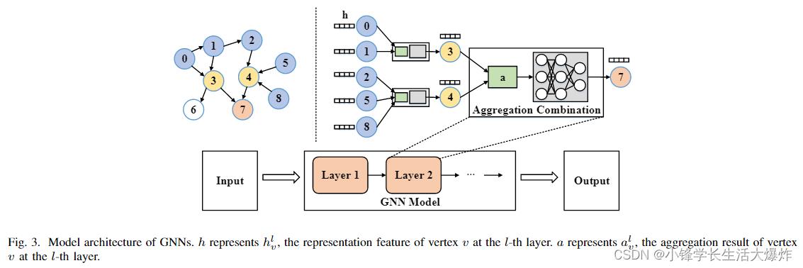
        As illustrated in Fig. 3, a GNN model consists of one or multiple layers consisting of neighbor aggregation and neural network operations, referred to as the Aggregation step and Combination step, respectively. In the Aggregation step, the Aggregate function Aggregate( ) is used to aggregate the feature vectors of in-coming neighboring vertices from the previous GNN layer for each target vertex. For example, in Fig. 3, vertex 4 would gather the feature vectors of itself and its incoming neighboring vertices (i.e., vertex 2, 5, 8) using the Aggregate function. In the Combination step, the Combine function Combine( ) transforms the aggregated feature vector of each vertex using neural network operations. To sum up, the aforementioned computation on a graph G(V, E) can be formally expressed by

        如图3所示，GNN模型由一个或多个层组成，包括邻居聚合和神经网络操作，分别称为聚合步骤和组合步骤。在聚合步骤中，聚合函数Aggregate()用于为每个目标顶点聚合来自前一个GNN层的传入相邻顶点的特征向量。例如，在图3中，顶点4将使用聚合函数收集其自身及其传入相邻顶点（即顶点2、5、8）的特征向量。在组合步骤中，组合函数Combine()使用神经网络操作变换每个顶点的聚合特征向量。综上所述，图G（V，E）上的上述计算可以形式化地表示为

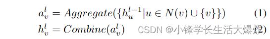
         where hl v denotes the feature vector of vertex v at the l-th layer, and N (v) represents the neighbors of vertex v. Specifically, the input feature of vertex v ∈ V is denoted as h0v .

        其中，hl v表示第l层顶点v的特征向量，N（v）表示顶点v的邻居。具体而言，顶点v∈v的输入特征表示为h0v。

C. Training Methods for Graph Neural Networks

        In this subsection, we introduce the training methods for GNNs, which are approached in two ways including full-batch training [69], [70] and mini-batch training [13], [71]–[74].

        在本小节中，我们介绍了GNN的训练方法，这两种方法包括全批训练[69]，[70]和小批训练[13]，[71]–[74]。

        A typical training procedure of neural networks, including GNNs, includes forward propagation and backward propagation. In forward propagation, the input data is passed through the layers of neural networks towards the output. Neural networks generate differences of the output of forward propagation by comparing it to the predefined labels. Then in backward propagation, these differences are propagated through the layers of neural networks in the opposite direction, generating gradients to update the model parameters.

        神经网络（包括GNN）的典型训练过程包括正向传播和反向传播。在正向传播中，输入数据通过神经网络层传递到输出端。神经网络通过将正向传播的输出与预定义的标签进行比较来产生正向传播输出的差异。然后在反向传播中，这些差异以相反的方向通过神经网络层传播，生成梯度以更新模型参数。

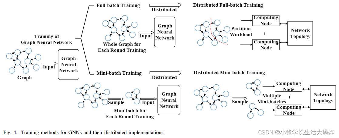
        As illustrated in Fig. 4, training methods of GNNs can be classified into full-batch training [69], [70] and mini-batch training [13], [71]–[74], depending on whether the whole graph is involved in each round. Here, we define a round of full-batch training consisting of a model computation phase, including forward and backward propagation, and a parameter update phase. On the other hand, a round in mini-batch training additionally contains a sampling phase, which samples a small-sized workload required for the subsequent model computation and thus locates prior to the other two phases. Thus, an epoch, which is defined as an entire pass of the data, is equivalent to a round of full-batch training, while that in mini-batch training usually contains several rounds. Details of these two methods are introduced below.

        如图4所示，GNN的训练方法可分为全批训练[69]、[70]和小批训练[13]、[71]–[74]，这取决于每一round是否涉及整个图形。这里，我们定义了一round完整的批量训练，包括模型计算阶段（包括正向和反向传播）和参数更新阶段。另一方面，一round小批量训练还包含采样阶段，该阶段对后续模型计算所需的小工作量进行采样，因此位于其他两个阶段之前。因此，被定义为整个数据传递的epoch相当于一轮完整的批量训练，而小批量训练中的epoch通常包含多round。下面将介绍这两种方法的详细信息。 

        1) Full-batch Training: Full-batch training utilizes the whole graph to update model parameters in each round.

        1）整批训练：整批训练利用整个图形来更新每一轮的模型参数。

        Given a training set Vt ⊂ V, the loss function of full-batch training is

        给定一个训练集Vt⊆V，全批训练的损失函数为

         where ∇l( ) is a loss function, yi is the known label of vertex vi, and zi is the output of GNN model when inputting feature xi of vi. In each epoch, GNN model needs to aggregate representations of all neighboring vertices for each vertex inVt all at once. As a result, the model parameters are updated only once at each epoch.

        其中，∇l( ) 是一个损失函数，yi是顶点vi的已知标号，zi是GNN模型在输入vi的特征xi时的输出。在每个epoch中，GNN模型需要一次聚合Vt中每个顶点的所有相邻顶点的表示。因此，模型参数在每个epoch仅更新一次。

        2) Mini-batch Training: Mini-batch training utilizes part of the vertices and edges in the graph to update model parameters in every forward propagation and backward propagation. It aims to reduce the number of vertices involved in the computation of one round to reduce the computing and memory resource requirements.

        2）小批量训练：小批量训练利用图形中的部分顶点和边来更新每个正向传播和反向传播中的模型参数。它旨在减少一轮计算中涉及的顶点数量，以减少计算和内存资源需求。

        Before each round of training, a mini-batch Vs is sampled from the training dataset Vt. By replacing the full training dataset Vt in equation (3) with the sampled mini-batch Vs, we obtain the loss function of mini-batch training:

        在每一轮训练之前，从训练数据集Vt中采样一个小批量Vs。通过将等式（3）中的完整训练数据集Vs替 换为采样的小批量Vs，我们获得了小批量训练的损失函数：

         It indicates that for mini-batch training, the model parameters are updated multiple times at each epoch, since numerous mini-batches are needed to have an entire pass of the training dataset, resulting in many rounds in an epoch. Stochastic Gradient Descent (SGD) [75], a variant of gradient descent which applies to mini-batch, is used to update the model parameters according to the loss L.

        它表明，对于小批量训练，模型参数在每个epoch被多次更新，因为需要许多小批量来完成训练数据集的整个过程，从而导致epoch中的许多轮。随机梯度下降（SGD）[75]，一种适用于小批量的梯度下降变体，用于根据损失L更新模型参数。

        Sampling: Mini-batch training requires a sampling phase to generate the mini-batches. The sampling phase first samples a set of vertices, called target vertices, from the training set according to a specific sampling strategy, and then it samples the neighboring vertices of these target vertices to generate a complete mini-batch. The sampling method can be generally categorized into three groups: Node-wise sampling, Layerwise sampling, and Subgraph-based sampling [56], [76].

        采样：小批量训练需要一个采样阶段来生成小批量。采样阶段首先根据特定的采样策略从训练集中采样一组顶点（称为目标顶点），然后对这些目标顶点的相邻顶点进行采样，以生成一个完整的小批量。采样方法通常可分为三组：节点采样、分层采样和基于子图的采样[56]，[76]。

小批量训练需要一个采样阶段来生成小批量。

        Node-wise sampling [13], [22], [77], [78] is directly applied to the neighbors of a vertex: the algorithm selects a subset of each vertex's neighbors. It is typical to specify a different sampling size for each layer. For example, in GraphSAGE [13], it samples at most 25 neighbors for each vertex in the first layer and at most 10 neighbors in the second layer.

        逐节点采样[13]，[22]，[77]，[78]直接应用于顶点的邻居：算法选择每个顶点邻居的子集。通常为每个层指定不同的采样大小。例如，在GraphSAGE[13]中，它为第一层中的每个顶点采样最多25个邻居，在第二层中采样最多10个邻居。

        Layer-wise sampling [71], [72], [79] enhances Nodewise sampling. It selects multiple vertices in each layer and then proceeds recursively layer by layer.

        逐层采样[71]、[72]、[79]增强了节点采样。它在每个层中选择多个顶点，然后逐层递归进行。

        Subgraph-based sampling [73], [80]–[82] first partition the original graph into multiple subgraphs, and then samples the mini-batches from one or a certain number of them.

        基于子图的采样[73]，[80]–[82]首先将原始图划分为多个子图，然后从其中的一个或一定数量的子图中对小批量进行采样。

TAXONOMY OF DISTRIBUTED GNN TRAINING

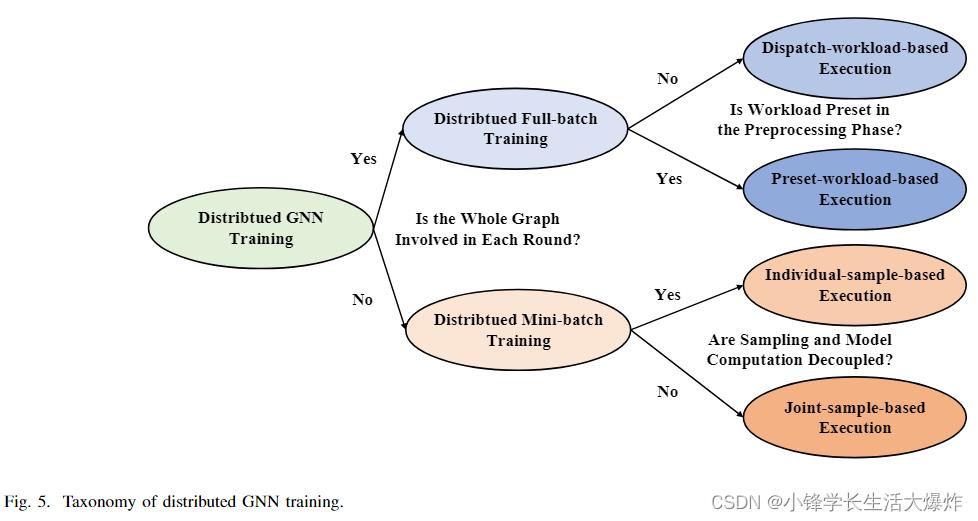
        This section introduces the taxonomy of distributed GNN training. As shown in Fig. 5, we firstly categorize it into distributed full-batch training and distributed mini-batch training, according to the training method introduced in Sec. II-C, i.e., whether the whole graph is involved in each round, and show the key differences between the two types. Each of the two types is classified further into two detailed types respectively by analyzing their workflows. This section introduces the firstlevel category, that is, distributed full-batch training and distributed mini-batch training, and makes a comparison between them. The second-level category of the two types will later be introduced in Sec. IV and Sec. V, respectively.

        本节介绍分布式GNN训练的分类。如图5所示，我们首先根据第II-C节中介绍的训练方法将其分为分布式全批量训练和分布式小批量训练，即每一轮是否涉及整个图，并显示了两种类型之间的关键差异。通过分析这两种类型的工作流程，将它们进一步分为两种详细类型。本节介绍了第一级类别，即分布式全批量训练和分布式小批量训练，并对它们进行了比较。这两种类型的第二级分类稍后将分别在第四节和第五节中介绍。

A. Distributed Full-batch Training

         Distributed full-batch training is the distributed implementation of GNN full-batch training, as illustrated in Fig. 4. Except for graph partition, a major difference is that multiple computing nodes need to synchronize gradients before updating model parameters, so that the models across the computing nodes remain unified. Thus, a round of distributed full-batch training includes two phases: model computation (forward propagation + backward propagation) and gradient synchronization. The model parameter update is included in the gradient synchronization phase.

        分布式全批训练是GNN全批训练的分布式实现，如图4所示。除了图分区之外，一个主要的区别是多个计算节点需要在更新模型参数之前同步梯度，以便计算节点之间的模型保持统一。因此，一轮分布式全批训练包括两个阶段：模型计算（正向传播+反向传播）和梯度同步。模型参数更新包括在梯度同步阶段中。

多个计算节点需要在更新模型参数之前同步梯度，以便计算节点之间的模型保持统一。

        Since each round involves the entire raw graph data, a considerable amount of computation and a large memory footprint are required in each round [37], [47], [50]. To deal with it, distributed full-batch training mainly adopts the workload partitioning method [44], [45]: split the graph to generate small workloads, and hand them over to different computing nodes.

        由于每一轮都涉及整个原始图形数据，因此每一轮[37]，[47]，[50]都需要大量的计算和大量的内存占用。为了解决这一问题，分布式全批训练主要采用工作负载划分方法[44]，[45]：分割图以生成小工作负载，并将其移交给不同的计算节点。

        Such a workflow leads to a lot of irregular inter-node communications in each round, mainly for transferring the features of vertices along the graph structure. This is because the graph data is partitioned and consequently stored in a distributed manner, and the irregular connection pattern in a graph, such as the arbitrary number and location of a vertices' neighbors. Therefore, many uncertainties exist in the communication of distributed full-batch training, including the uncertainty of the communication content, target, time, and latency, leading to challenges in the optimization of distributed full-batch training.

        这样的工作流在每一轮中都会导致大量不规则的节点间通信，主要是为了沿着图结构传递顶点的特征。这是因为图形数据被分割并因此以分布式方式存储，并且图形中的不规则连接模式，例如顶点的邻居的任意数量和位置。因此，分布式全批训练的通信中存在许多不确定性，包括通信内容、目标、时间和延迟的不确定性，导致分布式全批训练的优化面临挑战。

        As shown in Fig. 5, we further classify distributed fullbatch training more specifically into two categories according to whether the workload is preset in the preprocessing phase, namely dispatch-workload-based execution and presetworkload-based execution, as shown in the second column of Table III. Their detailed introduction and analysis are presented in Sec. IV-A and Sec. IV-B.

        如图5所示，根据预处理阶段是否预设了工作负载，我们进一步将分布式全批训练更具体地分为两类，即基于调度工作负载的执行和基于预任务负载的执行，如表III第二列所示。第IV-A节和第IV-B节对其进行了详细介绍和分析。

B. Distributed Mini-batch Training

        Similar to distributed full-batch training, distributed minibatch training is the distributed implementation of GNN minibatch training as in Fig. 4. It also needs to synchronize gradients prior to model parameter update, so a round of distributed mini-batch training includes three phases: sampling, model computation, and gradient synchronization. The model parameter update is included in the gradient synchronization phase.

        与分布式全批量训练类似，分布式小批量训练是GNN小批量训练的分布式实施，如图4所示。它还需要在模型参数更新之前同步梯度，因此一轮分布式小批量训练包括三个阶段：采样、模型计算和梯度同步。模型参数更新包括在梯度同步阶段中。

        Distributed mini-batch training parallelizes the training process by processing several mini-batches simultaneously, one for each computing node. The mini-batches can be sampled either by the computing node itself or by other devices, such as another node specifically for sampling. Each computing node performs forward propagation and backward propagation on its own mini-batch. Then, the nodes synchronize and accumulate the gradients, and update the model parameters accordingly. Such a process can be formulated by

        分布式小批量训练通过同时处理多个小批量（每个计算节点一个）来并行化训练过程。可以由计算节点本身或其他设备（例如专门用于采样的另一个节点）对小批量进行采样。每个计算节点在其自己的小批量上执行前向传播和后向传播。然后，节点同步并累积梯度，并相应地更新模型参数。该过程可通过以下方式制定：

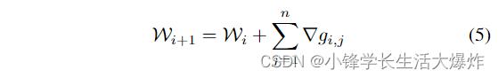
        where Wi is the weight parameters of model in the ith round of computation, ∇gi,j is the gradients generated in the backward propagation of the computing node j in the ith round of computation, and the n is the number of the computing nodes.

        其中Wi是第i轮计算中模型的权重参数，∇gi,j是第i次计算中计算节点j反向传播产生的梯度，n是计算节点的数量。

        As shown in Fig. 5, we further classify it more specifically into two categories according to whether the sampling and model computation are decoupled, namely individual-samplebased execution and joint-sample-based execution, as shown in the second column of Table III. Their detailed introduction and analysis are presented in Sec. V-A and Sec. V-B.

        如图5所示，根据采样和模型计算是否解耦，我们进一步将其更具体地分为两类，即基于单独样本的执行和基于联合样本的执行，如表III第二列所示。第V-A节和第V-B节对其进行了详细介绍和分析。

C. Comparison Between Distributed Full-batch Training and Distributed Mini-batch Training

        This subsection compares distributed full-batch training with distributed mini-batch training of GNNs. The major differences are also summarized in Table II.

        本小节比较了GNN的分布式全批量训练和分布式小批量训练。表二还总结了主要差异。

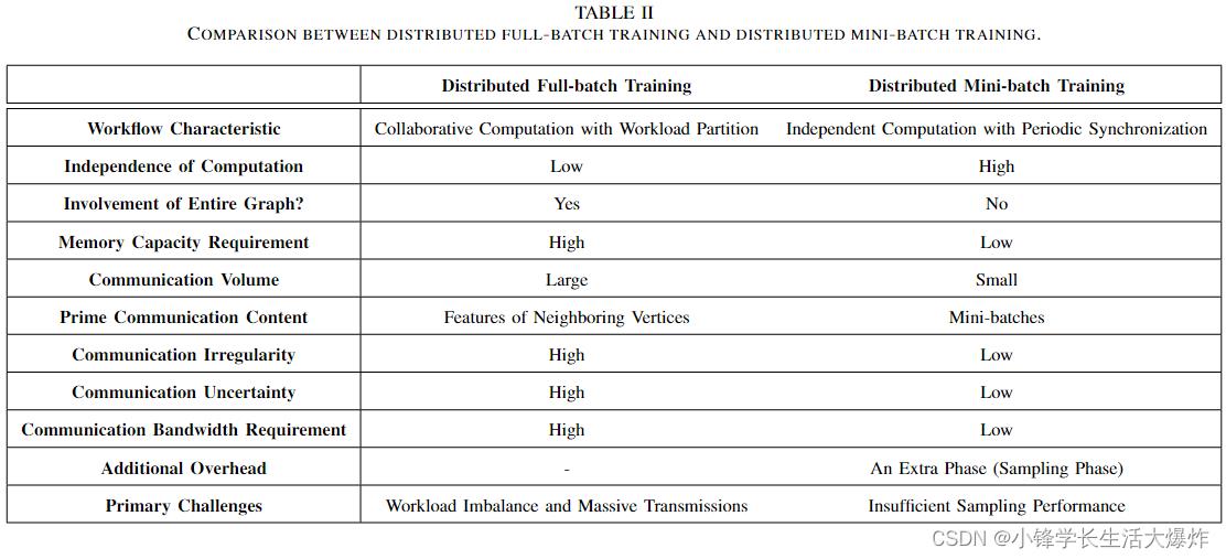
         The workflow of distributed full-batch training is summarized as collaborative computation with workload partition. Since the computation in each round involves the entire graph, the computing nodes need to cache it locally, leading to a high memory capacity requirement [44]. Also, the communication volume of distributed full-batch training is large [40], [47]. In every round, the Aggregate function needs to collect the features of neighbors for each vertex, causing a large quantity of inter-node communication requests since the graph is partitioned and stored on different nodes. Considering that the communication is based on the irregular graph structure, the communication irregularity of distributed full-batch training is high [46]. Another characteristic of communication is high uncertainty. The time of generating the communication request is indeterminate, since each computing node sends communication requests according to the currently involved vertices in its own computing process. As a result, the main challenges of distributed full batch training are workload imbalance and massive transmissions [45]–[47].

        分布式全批量训练的工作流程概括为具有工作负载划分的协同计算。由于每一轮的计算都涉及到整个图形，因此计算节点需要在本地缓存它，从而导致高内存容量需求[44]。此外，分布式全批量训练的通信量很大[40]，[47]。在每一轮中，Aggregate函数都需要收集每个顶点的邻居的特征，这会导致大量的节点间通信请求，因为图被划分并存储在不同的节点上。考虑到通信基于不规则图形结构，分布式全批量训练的通信不规则性很高[46]。通信的另一个特点是高度不确定性。生成通信请求的时间是不确定的，因为每个计算节点根据其自身计算过程中当前涉及的顶点发送通信请求。因此，分布式全批量训练的主要挑战是工作负载不平衡和大量传输[45]–[47]。

分布式全批量训练的主要挑战是工作负载不平衡和大量传输。

        In contrast, the workflow of distributed mini-batch training is summarized as independent computation with periodic synchronization. The major transmission content is the minibatches, sent from the sampling node (or component) to the computing node (or component) responsible for the current mini-batch [51], [52], [83]. As a result, these transmissions have low irregularity and low uncertainty, as the direction and content of transmission are deterministic. Since the computation of each round only involves the mini-batches, it triggers less communication volume and requires less memory capacity [51]. However, the extra sampling phase may cause some new challenges. Since the computation of the sampling phase is irregular and requires access to the whole graph for neighbor information of a given vertex, it is likely to encounter the problem of insufficient sampling performance, causing the subsequent computing nodes (or components) to stall due to lack of input, resulting in a performance penalty [56], [83].

        相比之下，分布式小批量训练的工作流被概括为具有周期同步的独立计算。主要传输内容是从采样节点（或组件）发送到负责当前小批量的计算节点（或部件）的小批量[51]，[52]，[83]。因此，这些传输具有低不规则性和低不确定性，因为传输的方向和内容是确定性的。由于每一轮的计算只涉及小批量，因此它触发的通信量更少，需要的内存容量也更少[51]。然而，额外的采样阶段可能会带来一些新的挑战。由于采样阶段的计算是不规则的，并且需要访问给定顶点的相邻信息的整个图，因此很可能会遇到采样性能不足的问题，导致后续计算节点（或组件）由于缺少输入而暂停，从而导致性能损失[56]，[83]。

D. Other Information of Taxonomy

        Table III provides a summary of the current studies on distributed GNN training using our proposed taxonomy. Except for the aforementioned classifications, we also add some supplemental information in the table to provide a comprehensive review of them.

        表III总结了使用我们提出的分类法进行分布式GNN训练的当前研究。除上述分类外，我们还在表中添加了一些补充信息，以对其进行全面审查。

        Software frameworks. The software frameworks used by the various studies are shown in the third column of Table III. PyTorch Geometric (PyG) [84] and Deep Graph Library (DGL) are the most popular among them. In addition, there are many newly proposed software frameworks aiming at distributed training of GNNs, and many of them are the optimization version of PyG [84] or DGL [85]. A detailed introduction to the software frameworks of distributed GNN training is presented in Sec. VI.

        软件框架。各种研究使用的软件框架如表III第三列所示。PyTorch Geometric（PyG）[84]和Deep Graph Library（DGL）是其中最受欢迎的。此外，有许多新提出的软件框架旨在对GNN进行分布式训练，其中许多是PyG[84]或DGL[85]的优化版本。第六节详细介绍了分布式GNN训练的软件框架。

        Hardware platforms. Multi-CPU platform and multi-GPU platform are the most common hardware platforms of distributed GNN training, as shown in the fourth column of Table III. Multi-CPU platform usually refers to a network with multiple servers, which uses CPUs as the only computing component. On the contrary, in multi-GPU platforms, GPUs are responsible for the major computing work, while CPU(s) handle some computationally complex tasks, such as workload partition and sampling. A detailed introduction to the hardware platforms is presented in Sec. VII.

        硬件平台。多CPU平台和多GPU平台是分布式GNN训练最常见的硬件平台，如表III第四列所示。多CPU平台通常指具有多个服务器的网络，其使用CPU作为唯一的计算组件。相反，在多GPU平台中，GPU负责主要的计算工作，而CPU处理一些计算复杂的任务，例如工作负载分区和采样。第七节详细介绍了硬件平台。

        Year. The contribution of distributed GNN training began to emerge in 2019 and is now showing a rapid growth trend. This is because more attention is paid to it due to the high demand from industry and academia to shorten the training time of GNN model.

        年份。分布式GNN培训的贡献在2019年开始显现，目前呈现快速增长趋势。这是因为工业界和学术界对缩短GNN模型训练时间的要求很高，因此越来越受到关注。

        Code available. The last column of Table III simply records the open source status of the corresponding study on distributed GNN training for the convenience of readers.

        代码可用。表III的最后一列简单地记录了分布式GNN训练的相应研究的开源状态，以方便读者。

IV. DISTRIBUTED FULL-BATCH TRAINING

        This section describes GNN distributed full-batch training in detail. Our taxonomy classifies it into two categories according to whether the workload is preset in the preprocessing phase, namely dispatch-workload-based execution and presetworkload-based execution, as shown in Fig. 6 (a).

        本节详细描述了GNN分布式全批量训练。我们的分类法根据预处理阶段是否预设了工作负载，将其分为两类，即基于调度工作负载的执行和基于预任务负载的执行，如图6（a）所示。

 A. Dispatch-workload-based Execution

        The dispatch-workload-based execution of distributed fullbatch training is illustrated in Fig. 6 (b). Its workflow, computational pattern, communication pattern, and optimization techniques are introduced in detail as follows.

        图6（b）说明了分布式全批次训练的基于调度工作量的执行。其工作流程、计算模式、通信模式和优化技术详细介绍如下。

        1) Workflow: In the dispatch-workload-based execution, a leader and multiple workers are used to perform training. The leader stores the model parameters and the graph data, and is also responsible for scheduling: it splits the computing workloads into chunks, distributes them to the workers, and collects the intermediate results sent from the workers. It also processes these results and advances the computation. Note that, the chunk we use here is as a unit of workload.

        1） 工作流：在基于调度工作负载的执行中，使用一名leader和多名workers进行训练。领导者存储模型参数和图形数据，还负责调度：它将计算工作负载分割成chunk，分发给工作人员，并收集工作人员发送的中间结果。它还处理这些结果并推进计算。注意，我们这里使用的chunk是工作负载的一个单位。

        2) Computational Pattern: The computational patterns of forward propagation and backward propagation are similar in dispatch-workload-based execution: the latter can be seen as the reversed version of the former. As a result, we only introduce forward propagation's computational pattern here for simplicity. The patterns of the two functions in forward propagation (Aggregate and Combine) differ a lot and will be introduced below respectively.

        2） 计算模式：前向传播和后向传播的计算模式在基于调度工作负载的执行中是相似的：后者可以被视为前者的相反版本。因此，为了简单起见，我们只在这里引入前向传播的计算模式。前向传播中两个函数（Aggregate和Combine）的模式有很大不同，下面将分别介绍。

        Aggregate function. The computational pattern of the Aggregate function is dynamic and irregular, making workload partition for this step a challenge. In the Aggregation step, each vertex needs to aggregate the features of its own neighbors. As a result, the computation of the Aggregation step relies heavily on the graph structure, which is irregular or even changeable. Thus, the number and memory location of neighbors vary significantly among vertices, resulting in the dynamic and irregular computational pattern [86], causing the poor workload predictability and aggravating the difficulty of workload partition.

        聚合函数。聚合函数的计算模式是动态的和不规则的，这使得这一步骤的工作负载划分成为一个挑战。在聚合步骤中，每个顶点都需要聚合其自身邻居的特征。因此，聚合步骤的计算严重依赖于不规则甚至可变的图形结构。因此，相邻节点的数量和内存位置在顶点之间显著不同，导致动态和不规则的计算模式[86]，导致工作负载可预测性差，并加剧了工作负载划分的难度。

        Combine function. The computational pattern of the Combine function is static and regular, thus the workload partition for it is simple. The computation of the Combination step is to perform neural network operations on each vertex. Since the structure of neural networks is regular and these operations share the same weight parameters, the Combination step enjoys a regular computational pattern. Consequently, a simple partitioning method is sufficient to maintain workload balance, so it is relatively not a major consideration in dispatch-workload-based execution of GNN distributed fullbatch training.

        组合函数。Combine函数的计算模式是静态的和规则的，因此它的工作负载划分很简单。组合步骤的计算是对每个顶点执行神经网络操作。由于神经网络的结构是规则的，并且这些操作共享相同的权重参数，因此组合步骤具有规则的计算模式。因此，简单的分区方法足以保持工作负载平衡，因此在GNN分布式全批训练的基于调度工作负载的执行中，它相对不是主要考虑因素。

。。。