[论文阅读-1]ImageNet Classification with Deep Convolutional Neural Networks

Posted 2023-04-25

参考技术A

Abstract

我们训练了一个大型的深度卷积神经网络，将ImageNet lsvprc -2010竞赛中的120万幅高分辨率图像分类为1000个不同的类。在测试数据上，我们实现了top-1和top-5的错误率，分别为37.5%和17.0%，这与前的最高水平相比有了很大的提高。该神经网络有6000万个参数和65万个神经元，由5个卷积层(其中一些后面接了最大池化层)和3个全连接层(最后的1000路softmax)组成。为了使训练更快，我们使用了非饱和神经元和一个非常高效的GPU实现卷积运算。为了减少全连通层的过拟合，我们采用了一种最近发展起来的正则化方法——dropout，结果显示它非常有效。我们还在ILSVRC-2012比赛中输入了该模型的一个变体，并获得了15.3%的top-5测试错误率，而第二名获得了26.2%的错误率.

1 Introduction

当前的物体识别方法主要利用机器学习方法。为了提高它们的性能，我们可以收集更大的数据集，学习更强大的模型，并使用更好的技术来防止过度拟合。直到最近，标记图像的数据集在成千上万的图像(例如，NORB [16]， Caltech-101/256 [8,9]， CIFAR-10/100[12])中相对较小。使用这种大小的数据集可以很好地解决简单的识别任务，特别是如果使用保存标签的转换来扩展它们。例如，MNIST数字识别任务的当前最佳错误率(<0.3%)接近人类性能[4]。但是现实环境中的物体表现出相当大的可变性，所以为了学会识别它们，有必要使用更大的训练集。的确，小图像数据集的缺点已经被广泛认识(例如，Pinto等人的[21])，但直到最近才有可能收集数百万张图像的标记数据集。新的更大的数据集包括LabelMe[23]，它由成千上万的全分段图像组成，和ImageNet[6]，它由超过22000个类别的超过1500万标记的高分辨率图像组成。

要从数百万张图像中了解数千个物体，我们需要一个具有巨大学习能力的模型。
然而，对象识别任务的巨大复杂性意味着即使像ImageNet这样大的数据集也无法指定这个问题，因此我们的模型也应该具有大量的先验知识来补偿我们没有的所有数据。卷积神经网络(Convolutional neural networks, CNNs)就是这样一类模型[16,11,13,18,15,22,26]。它们的能力可以通过改变深度和宽度来控制，而且它们还对图像的性质(即统计的平稳性和像素依赖的局部性)做出了强有力且最正确的假设。
因此，与具有相似大小层的标准前馈神经网络相比，CNNs具有更少的连接和参数，因此更容易训练，而其理论上最好的性能可能只会稍微差一些。

尽管CNNs的质量很吸引人，尽管它们的本地架构相对高效，但在高分辨率图像上大规模应用仍然非常昂贵。幸运的是，当前的gpu与高度优化的2D卷积实现相结合，已经足够强大，可以方便地训练有趣的大型CNNs，而最近的数据集(如ImageNet)包含了足够多的标记示例，可以在不严重过拟合的情况下训练此类模型。

本文的具体贡献如下：

最后，网络的大小主要受到当前gpu上可用内存的大小和我们愿意忍受的训练时间的大小的限制。我们的网络需要5到6天的时间来训练两个GTX 580 3GB GPU。我们所有的实验都表明，只要等待更快的gpu和更大的数据集可用，我们的结果就可以得到改善。

2 The Dataset

ImageNet是一个包含超过1500万张高分辨率图像的数据集，属于大约22000个类别。这些图片是从网上收集来的，并由人工贴标签者使用亚马逊的土耳其机械众包工具进行标记。从2010年开始，作为Pascal视觉对象挑战赛的一部分，每年都会举办一场名为ImageNet大型视觉识别挑战赛(ILSVRC)的比赛。ILSVRC使用ImageNet的一个子集，每个类别大约有1000张图片。总共大约有120万张训练图像、5万张验证图像和15万张测试图像。

ILSVRC-2010 是唯一可用测试集标签的 ILSVRC 版本，因此这是我们进行大多数实验的版本。由于我们也在 ILSVRC-2012 竞赛中加入了我们的模型，在第6节中，我们也报告了我们在这个版本的数据集上的结果，对于这个版本的数据集，测试集标签是不可用的。在 ImageNet 上，通常报告两个错误率：top-1 和 top-5，其中 top-5 错误率是测试图像的一部分，其中正确的标签不在模型认为最可能的五个标签中。

ImageNet由可变分辨率的图像组成，而我们的系统需要一个恒定的输入维数。
因此，我们将图像降采样到256 * 256的固定分辨率。给定一个矩形图像，我们首先重新调整图像的大小，使其短边长度为256，然后从结果图像中裁剪出中心的256%256块。除了从每个像素中减去训练集上的平均活动外，我们没有以任何其他方式对图像进行预处理。因此，我们将网络训练成像素的原始RGB值(居中)。

3 The Architecture

3.1 ReLU Nonlinearity

3.2 Training on Multiple GPUs

3.3 Local Response Normalization

3.4 Overlapping Pooling

Pooling layers in CNNs summarize the outputs of neighboring groups of neurons in the same kernel map. Traditionally, the neighborhoods summarized by adjacent pooling units do not overlap (e.g.,[17, 11, 4]). To be more precise, a pooling layer can be thought of as consisting of a grid of pooling units spaced s pixels apart, each summarizing a neighborhood of size z z centered at the location of the pooling unit. If we set s = z, we obtain traditional local pooling as commonly employed in CNNs. If we set s < z, we obtain overlapping pooling. This is what we use throughout our network, with s = 2 and z = 3. This scheme reduces the top-1 and top-5 error rates by 0.4% and 0.3%, respectively, as compared with the non-overlapping scheme s = 2; z = 2, which produces output of equivalent dimensions. We generally observe during training that models with overlapping pooling find it slightly more difficult to overfit.

3.5 Overall Architecture

Now we are ready to describe the overall architecture of our CNN. As depicted in Figure 2, the net contains eight layers with weights; the first five are convolutional and the remaining three are fully-connected. The output of the last fully-connected layer is fed to a 1000-way softmax which produces a distribution over the 1000 class labels. Our network maximizes the multinomial logistic regression objective, which is equivalent to maximizing the average across training cases of the log-probability of the correct label under the prediction distribution.

4 Reducing Overfitting

4.1 Data Augmentation

4.2 Dropout

结合许多不同模型的预测是减少测试错误的一种非常成功的方法[1,3]，但是对于已经需要几天训练的大型神经网络来说，这似乎太昂贵了。然而，有一个非常有效的模型组合版本，它在训练期间只花费大约2倍的成本。最近介绍的技术称为dropout[10]，它将每个隐藏神经元的输出设置为0，概率为0.5。以这种方式丢弃的神经元不参与正向传递，也不参与反向传播。所以每次输入时，神经网络都会对不同的结构进行采样，但是所有这些结构都共享权重。这种技术减少了神经元之间复杂的相互适应，因为神经元不能依赖于特定的其他神经元的存在。因此，它被迫学习与其他神经元的许多不同随机子集结合使用的更健壮的特征。在测试时，我们使用所有的神经元，但将它们的输出乘以0.5，这是一个合理的近似值，近似于取由指数型多退出网络产生的预测分布的几何平均值。

我们在图2的前两个完全连接的层中使用了dropout。没有dropout，我们的网络显示出大量的过拟合。Dropout使收敛所需的迭代次数增加了一倍。

5 Details of learning

7 Discussion

经典网络模型 ResNet-50 在 ImageNet-1k 上的研究 | 实验笔记+论文解读

需要 ImageNet-1k 数据集的来这篇博文: https://blog.csdn.net/qq_39377134/article/details/103128970
但是要准备好 240 GB 大小的磁盘空间哈，因为数据集压缩包是 120 GB 多一些。

本文是关于 ResNet-50 在 ImageNet 上的实验研究，目前的话，实验数据集分别是 ImageNet-240 和 ImageNet-1k，其中前者是后者的一个子集。

接下来直接上实验结果吧，第一次实验，我是 freeze all layer exclude last layer，注意此处我加载了在 ImageNet-1k 上预训练的模型，实验结果是: train_acc = 93.8, val_acc = 93.44, test_acc = 93.48。

第二次实验(这一次实验加载的预训练模型是加载第一次保存下来的模型，原因是我们要在第一次训练完 last layer参数的情况下做微调，而不是直接 unfreeze layer4 和 fc layer，这样会破坏预训练学习到的信息，这里还要提一下，微调的话，学习率最好是第一次训练的 1/10)，我是 freeze all layer exclude layer4 and fc layer(也就是上面说的 last layer)，实验结果是: train_acc = 95.24，val_acc = 93.6，test_acc = 93.7。对比第一次和第二次的实验结果，我们可以发现在 val 和 test 上获得了些许提升，但是从 train 可以看出开始过拟合了。

第三次实验(这一次实验加载的预训练模型是加载第一次保存下来的模型)，我是 freeze all layer exclude layer3 and layer4 and fc layer，实验结果是: train_acc = 95.81, val_acc = 93.67, test_acc = 93.9，对比第三次实验和第一次实验，可以发现，unfreeze 更多的网络层数，能略微提升准确率，但是也不太多吧。

对于过拟合，我说说我的看法吧，加大数据量可以缓解过拟合，但也仅仅只是缓解，除非你的数据集包含了所有现实情况，不然这个无法避免，我们能做的只是缩小 train_acc 和 val_acc 之间的 gap。

最后再说一下在 ImageNet-1k 上的 acc = 87.43，对比 ImageNet-240 和 ImageNet-1k 上的结果，我们可以发现，模型在 ImageNet-1k 上做 pre-train，然后 transfer 到 ImageNet-240 上，可以明显提升模型效果，不过两者都是同属于一个 domain，我们需要更多的在不同 domain 上测试 transfer 的效果才行。

对于数据量和模型泛化性的研究，有一篇论文写的很好，Big Transfer (BiT): General Visual Representation Learning，该论文在 ImageNet-1k(1.28M 张图片)，ImageNet-21k(14.2M 张图片)，JFT-300M(300M 张图片)，上分别实验，发现数据量越大，效果越好，可以在 papers with code 上的 benckmark 查到 ResNet-50 在 ImageNet-1k 上的 test_acc = 77.15，但是在 JFT-300M 上做预训练之后，再做 transfer 的话，可以达到 test_acc = 87.54。这里又不得不感慨，大力出奇迹，只是这次换成了数据集。。。。。

想了下，还是要放代码的，我这里放一下 train.py:

import torch

from utils.eval import calc_acc
from utils.utils import setup_seed, get_dataloader, show_img, predict_batch, set_gpu
from utils.model import define_model, define_optim, start_train
from torch import nn

# 设置哪块显卡可见
device = set_gpu('0, 1')

# 设置随机数种子，使结果可复现
setup_seed(20)

# 数据读取
train_batch = 160
test_batch = 160
EPOCH = 200
trainloader, testloader, classes = get_dataloader(train_batch, test_batch)

# 对训练集的一个batch图片进行展示
show_img(trainloader, classes, batch_size=train_batch)

# 网络结构定义
net = define_model(classes)
net = nn.DataParallel(net)
net.to(device)

# 定义优化器和损失函数
criterion, optimizer = define_optim(net)
net.load_state_dict(torch.load('resnetV1-50-9519-93.pth'))

# 开始模型训练
start_train(net, EPOCH, trainloader, device, optimizer, criterion, testloader)

# 训练后在测试集上进行评测
net.load_state_dict(torch.load('resnet50Cls.pth'))
print(calc_acc(net, testloader, device))

# 进行模型预测
predict_batch(net, testloader, classes, test_batch, device)

完整代码的话，我放到 Github了: https://github.com/MaoXianXin/PycharmProjects

补充论文解读: Deep Residual Learning for Image Recognition，主要解决网络加深，模型优化困难问题。
Deeper neural networks are more difficult to train. We present a residual learning framework to ease the training of networks that are substantially deeper than those used previously.

解读: 训练深度神经网络是困难的，当然浅层的网络不困难，该篇论文提出残差学习架构来解决该问题。

We explicitly reformulate the layers as learning residual functions with reference to the layer inputs, instead of learning unreferenced functions.

解读: 这里可以理解为引入残差连接。

The depth of representations is of central importance for many visual recognition tasks.

Deep networks naturally integrate low/mid/high-level features and classifiers in an end-to-end multi-layer fashion, and the “levels” of features can be enriched by the number of stacked layers(depth).

解读: 对于很多视觉识别任务来说，网络的深度是非常重要的，可以理解为分别提取到 low/mid/high 三种层次的特征。

Driven by the significance of depth, a question arises: Is learning better networks as easy as stacking more layers ? An obstacle to answering this question was the notorious problem of vanishing/exploding gradients, which hamper convergence from the beginning. This problem, however, has been largely addressed by normalized initialization and intermediate normalization layers, which enable networks with tens of layers to start converging for stochastic gradient descent(SGD) with back-propagation.

解读: 对于验证模型深度越深，网络的性能是否越好之前，这里还存在一个阻碍，就是梯度消失和爆炸，不过这个问题很大程度上可以通过正则初始化以及中间正则化层解决。

When deeper networks are able to start converging, a degradation problem has been exposed: with the network depth increasing, accuracy gets saturated and then degrades rapidly. Unexpectedly, such degradation is not caused by overfitting, and adding more layers to a suitably deep model leads to higher training error.

The degradation(of training accuracy) indicates that not all systems are similarly easy to optimize.

解读: 在解决了网络的梯度消失和爆炸之后，我们的网络可以正常的收敛了，但是随着网络加深，出现了准确率饱和以及快速退化的问题，并且这个问题不是由过拟合造成的。我们还可以这样理解，对于一个适当深度的网络，如果你在这个基础之上再添加层数，这个时候你不会获得更好的性能，反而会得到更大的误差。

We hypothesize that it is easier to optimize the residual mapping than to optimize the original, unreferenced mapping.

解读: 这个假设是这篇论文的关键，也是提出 residual mapping 的立足点。

To the extreme, if an identity mapping were optimal, it would be easier to push the residual to zero than to fit an identity mapping by a stack of nonlinear layers.

疑惑: 还不是特别理解，待后面解决吧。目前的理解就是，优化添加了残差连接的网络比直接优化堆叠起来的非线性层更容易。

In our case, the shortcut connections simply perform identity mapping, and their outputs are added to the outputs of the stacked layers. Identity shortcut connections add neither extra parameter nor computational complexity. The entire network can still be trained end-to-end by SGD with backpropagation, and can be easily implemented using common libraries.

解读: 此处提到的 identity mapping 既不增加额外的参数，也不增加计算复杂度。

We evaluate our method on the ImageNet 2012 classification dataset that consists of 1000 classes. The models are trained on the 1.28 million training images, and evaluated on the 50k validation images. We also obtain a final result on the 100k test images, reported by the test server.

解读: ResNet 模型是在 ImageNet 2012，可以称为 ImageNet-1k 数据集上训练的，有 1.28M 张训练图片，50k 张验证图片，以及 100k 张测试图片。

we also note that the 18-layer plain/residual nets are comparably accurate, but the 18-layer ResNet converges faster.

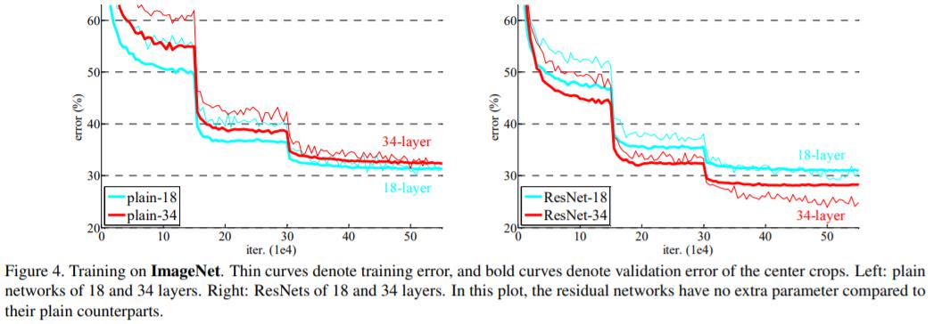
解读: 从上图，确实可以看出 ResNet-18 在初始阶段收敛速度快于 Plain-18。

Bottleneck Architectures: a stack of 3 layers, 1x1, 3x3, and 1x1 convolutions, where the 1x1 layers are responsible for reducing and then increasing(restoring) dimensions leaving the 3x3 layer a bottleneck with smaller input/output dimensions.

The parameter-free identity shortcuts are particularly important for the bottleneck architectures. If the identity shortcut is replaced with projection, one can show that the time complexity and model size are doubled, as the shortcut is connected to the two high-dimensional ends. So identity shortcuts lead to more efficient models for the bottleneck designs.

解读: 此处说的是 Bottleneck 的结构，两端是 1x1，中间是 3x3，同时两端的 dimension 大，中间的 dimension 小，可以节省参数量和计算量

The 50/101/152-layer ResNets are more accurate than the 34-layer ones by considerable margins.

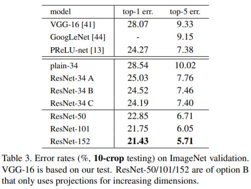
解读: 从上图确实可以看出来 50/101/152 层的 ResNet 准确率比 34 层的高。

We also notice that the deeper ResNet has smaller magnitudes of responses, as evidenced by the comparisons among ResNet-20, 56, and 110. When there are more layers, an individual layer of ResNets tends to modify the signal less.

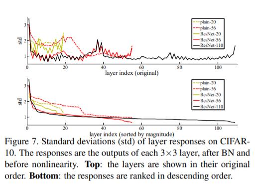
解读: 此处展示不同网络的各个层的 magnitudes of responses