KITTI数据集可视化：点云多种视图的可视化实现

Posted 2023-04-12 Clichong

---

如有错误，恳请指出。

---

在本地上，可以安装一些软件，比如：Meshlab，CloudCompare等3D查看工具来对点云进行可视化。而这篇博客是将介绍一些代码工具将KITTI数据集进行可视化操作，包括点云鸟瞰图，FOV图，以及标注信息在图像+点云上的显示。

文章目录

• 1. 数据集准备
• 2. 环境准备
• 3. KITTI数据集可视化
• 4. 点云可视化
• 5. 鸟瞰图可视化

1. 数据集准备

KITTI数据集作为自动驾驶领域的经典数据集之一，比较适合我这样的新手入门。以下资料是为了实现对KITTI数据集的可视化操作。首先在官网下载对应的数据：http://www.cvlibs.net/datasets/kitti/eval_object.php?obj_benchmark=3d，下载后数据的目录文件结构如下所示：

├── dataset
│   ├── KITTI
│   │   ├── object
│   │   │   ├──KITTI
│   │   │      ├──ImageSets
│   │   │   ├──training
│   │   │      ├──calib & velodyne & label_2 & image_2

---

2. 环境准备

这里使用了一个kitti数据集可视化的开源代码：https://github.com/kuixu/kitti_object_vis，按照以下操作新建一个虚拟环境，并安装所需的工具包。其中千万不要安装python3.7以上的版本，因为vtk不支持。

# 新建python=3.7的虚拟环境
conda create -n kitti_vis python=3.7 # vtk does not support python 3.8
conda activate kitti_vis

# 安装opencv, pillow, scipy, matplotlib工具包
pip install opencv-python pillow scipy matplotlib

# 安装3D可视化工具包（以下指令会自动安转所需的vtk与pyqt5）
conda install mayavi -c conda-forge

# 测试
python kitti_object.py --show_lidar_with_depth --img_fov --const_box --vis

---

3. KITTI数据集可视化

下面依次展示 KITTI 数据集可视化结果，这里通过设置 data_idx=10 来展示编号为000010的数据，代码中dataset需要修改为数据集实际路径。（最后会贴上完整代码）

def visualization():
    import mayavi.mlab as mlab
    dataset = kitti_object(os.path.join(ROOT_DIR, '../dataset/KITTI/object'))
    
    # determine data_idx
    data_idx = 100
    
    # Load data from dataset
    objects = dataset.get_label_objects(data_idx) 
    print("There are %d objects.", len(objects))
    img = dataset.get_image(data_idx)             
    img = cv2.cvtColor(img, cv2.COLOR_BGR2RGB)
    img_height, img_width, img_channel = img.shape 
    pc_velo = dataset.get_lidar(data_idx)[:,0:3]  
    calib = dataset.get_calibration(data_idx)   

代码来源于参考资料，在后面会贴上我自己修改的测试代码。以下包含9种可视化的操作：

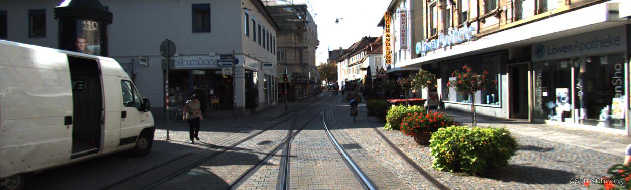
• 1. 图像显示

def show_image(self):
    Image.fromarray(self.img).show()
    cv2.waitKey(0)

结果展示：

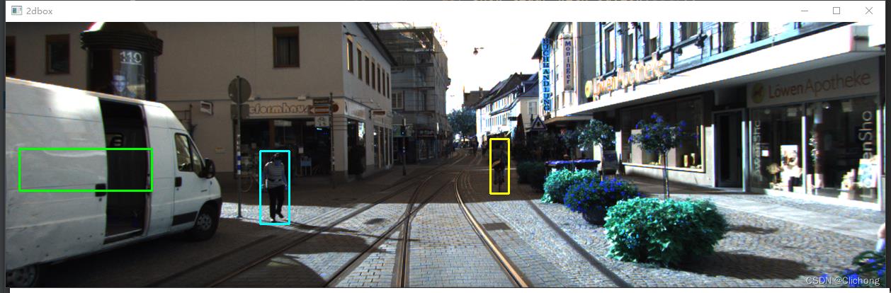
• 2. 图片上绘制2D bbox

    def show_image_with_2d_boxes(self):
        show_image_with_boxes(self.img, self.objects, self.calib, show3d=False)
        cv2.waitKey(0)

结果展示：

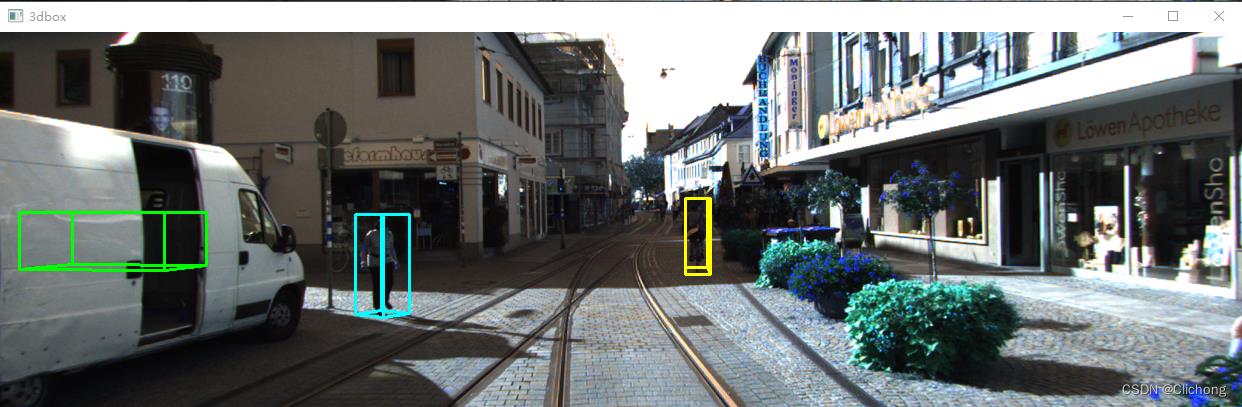
• 3. 图片上绘制3D bbox

    def show_image_with_3d_boxes(self):
        show_image_with_boxes(self.img, self.objects, self.calib, show3d=True)
        cv2.waitKey(0)

结果展示：

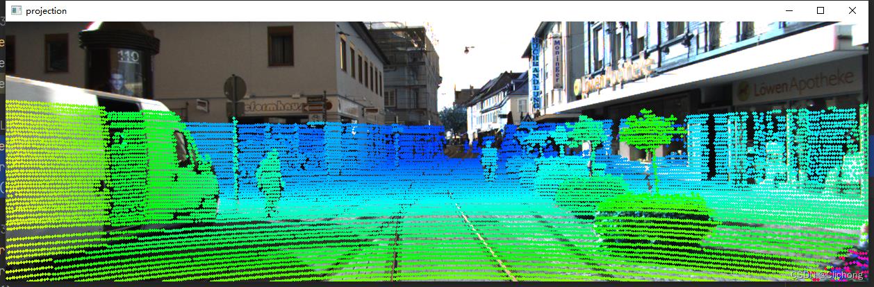
• 4. 图片上绘制Lidar投影

    def show_image_with_lidar(self):
        show_lidar_on_image(self.pc_velo, self.img, self.calib, self.img_width, self.img_height)
        mlab.show()

结果展示：

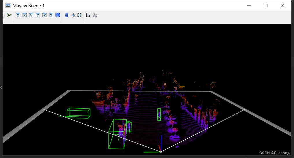
• 5. Lidar绘制3D bbox

    def show_lidar_with_3d_boxes(self):
        show_lidar_with_boxes(self.pc_velo, self.objects, self.calib, True, self.img_width, self.img_height)
        mlab.show()

结果展示：

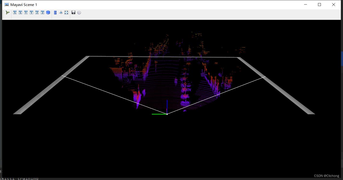
• 6. Lidar绘制FOV图

    def show_lidar_with_fov(self):
        imgfov_pc_velo, pts_2d, fov_inds = get_lidar_in_image_fov(self.pc_velo, self.calib,
                                                                  0, 0, self.img_width, self.img_height, True)
        draw_lidar(imgfov_pc_velo)
        mlab.show()

结果展示：

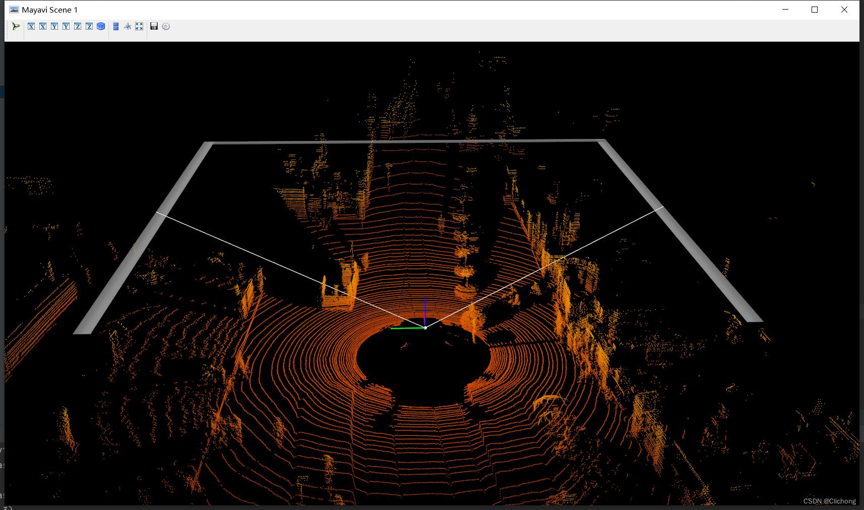
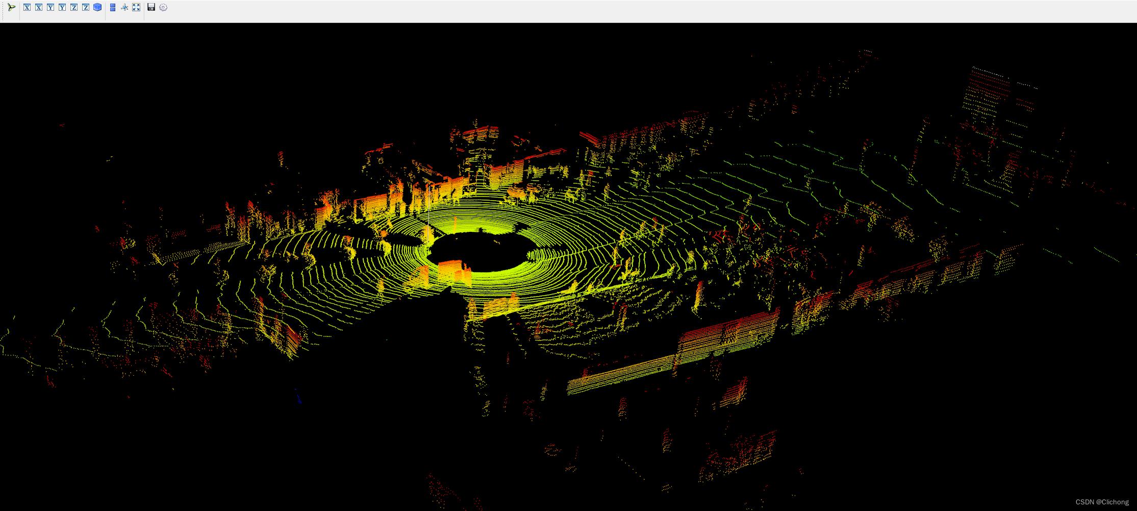
• 7. Lidar绘制3D图

    def show_lidar_with_3dview(self):
        draw_lidar(self.pc_velo)
        mlab.show()

结果展示：

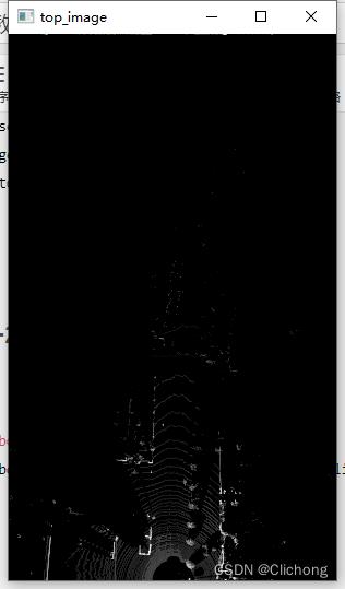
• 8. Lidar绘制BEV图

BEV图的显示与其他视图不一样，这里的代码需要有点改动，因为这里需要lidar点云的其他维度信息，所以输入不仅仅是xyz三个维度。改动代码：

# 初始
pc_velo = dataset.get_lidar(data_idx)[:, 0:3]

# 改为（要增加其他维度才可以查看BEV视图）
pc_velo = dataset.get_lidar(data_idx)[:, 0:4]

测试代码：

    def show_lidar_with_bev(self):
        from kitti_util import draw_top_image, lidar_to_top
        top_view = lidar_to_top(self.pc_velo)
        top_image = draw_top_image(top_view)
        cv2.imshow("top_image", top_image)
        cv2.waitKey(0)

结果展示：

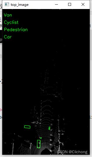
• 9. Lidar绘制BEV图+2D bbox

同样，这里的代码改动与3.8节一样，需要点云的其他维度信息

    def show_lidar_with_bev_2d_bbox(self):
        show_lidar_topview_with_boxes(self.pc_velo, self.objects, self.calib)
        mlab.show()

结果展示：

• 完整测试代码

参考代码：

import mayavi.mlab as mlab
from kitti_object import kitti_object, show_image_with_boxes, show_lidar_on_image, \\
    show_lidar_with_boxes, show_lidar_topview_with_boxes, get_lidar_in_image_fov, \\
    show_lidar_with_depth
from viz_util import draw_lidar
import cv2
from PIL import Image
import time

class visualization:
    # data_idx: determine data_idx
    def __init__(self, root_dir=r'E:\\Study\\Machine Learning\\Dataset3d\\kitti', data_idx=100):
        dataset = kitti_object(root_dir=root_dir)

        # Load data from dataset
        objects = dataset.get_label_objects(data_idx)
        print("There are  objects.".format(len(objects)))
        img = dataset.get_image(data_idx)
        img = cv2.cvtColor(img, cv2.COLOR_BGR2RGB)
        img_height, img_width, img_channel = img.shape
        pc_velo = dataset.get_lidar(data_idx)[:, 0:3]  # 显示bev视图需要改动为[:, 0:4]
        calib = dataset.get_calibration(data_idx)

        # init the params
        self.objects = objects
        self.img = img
        self.img_height = img_height
        self.img_width = img_width
        self.img_channel = img_channel
        self.pc_velo = pc_velo
        self.calib = calib

    # 1. 图像显示
    def show_image(self):
        Image.fromarray(self.img).show()
        cv2.waitKey(0)

    # 2. 图片上绘制2D bbox
    def show_image_with_2d_boxes(self):
        show_image_with_boxes(self.img, self.objects, self.calib, show3d=False)
        cv2.waitKey(0)

    # 3. 图片上绘制3D bbox
    def show_image_with_3d_boxes(self):
        show_image_with_boxes(self.img, self.objects, self.calib, show3d=True)
        cv2.waitKey(0)

    # 4. 图片上绘制Lidar投影
    def show_image_with_lidar(self):
        show_lidar_on_image(self.pc_velo, self.img, self.calib, self.img_width, self.img_height)
        mlab.show()

    # 5. Lidar绘制3D bbox
    def show_lidar_with_3d_boxes(self):
        show_lidar_with_boxes(self.pc_velo, self.objects, self.calib, True, self.img_width, self.img_height)
        mlab.show()

    # 6. Lidar绘制FOV图
    def show_lidar_with_fov(self):
        imgfov_pc_velo, pts_2d, fov_inds = get_lidar_in_image_fov(self.pc_velo, self.calib,
                                                                  0, 0, self.img_width, self.img_height, True)
        draw_lidar(imgfov_pc_velo)
        mlab.show()

    # 7. Lidar绘制3D图
    def show_lidar_with_3dview(self):
        draw_lidar(self.pc_velo)
        mlab.show()

    # 8. Lidar绘制BEV图
    def show_lidar_with_bev(self):
        from kitti_util import draw_top_image, lidar_to_top
        top_view = lidar_to_top(self.pc_velo)
        top_image = draw_top_image(top_view)
        cv2.imshow("top_image", top_image)
        cv2.waitKey(0)

    # 9. Lidar绘制BEV图+2D bbox
    def show_lidar_with_bev_2d_bbox(self):
        show_lidar_topview_with_boxes(self.pc_velo, self.objects, self.calib)
        mlab.show()


if __name__ == '__main__':
    kitti_vis = visualization()
    # kitti_vis.show_image()
    # kitti_vis.show_image_with_2d_boxes()
    # kitti_vis.show_image_with_3d_boxes()
    # kitti_vis.show_image_with_lidar()
    # kitti_vis.show_lidar_with_3d_boxes()
    # kitti_vis.show_lidar_with_fov()
    # kitti_vis.show_lidar_with_3dview()
    # kitti_vis.show_lidar_with_bev()
    kitti_vis.show_lidar_with_bev_2d_bbox()

    # print('...')
    # cv2.waitKey(0)

此外，下面再提供两份可视化代码。

---

4. 点云可视化

这里的同样使用的是上述的图例，且直接输入的KITTI数据集的.bin文件，即可显示点云图像。

• 参考代码：

import numpy as np
import mayavi.mlab
import os

# 000010.bin这里需要填写文件的位置
# bin_file = '../data/object/training/velodyne/000000.bin'
# assert os.path.exists(bin_file), " is not exists".format(bin_file)

kitti_file = r'E:\\Study\\Machine Learning\\Dataset3d\\kitti\\training\\velodyne\\000100.bin'
pointcloud = np.fromfile(file=kitti_file, dtype=np.float32, count=-1).reshape([-1, 4])
# pointcloud = np.fromfile(str("000010.bin"), dtype=np.float32, count=-1).reshape([-1, 4])

print(pointcloud.shape)
x = pointcloud[:, 0]  # x position of point
y = pointcloud[:, 1]  # y position of point
z = pointcloud[:, 2]  # z position of point
r = pointcloud[:, 3]  # reflectance value of point
d = np.sqrt(x ** 2 + y ** 2)  # Map Distance from sensor

vals = 'height'
if vals == "height":
    col = z
else:
    col = d

fig = mayavi.mlab.figure(bgcolor=(0, 0, 0), size=(640, 500))
mayavi.mlab.points3d(x, y, z,
                     col,  # Values used for Color
                     mode="point",
                     colormap='spectral',  # 'bone', 'copper', 'gnuplot'
                     # color=(0, 1, 0),   # Used a fixed (r,g,b) instead
                     figure=fig,
                     )

x = np.linspace(5, 5, 50)
y = np.linspace(0, 0, 50)
z = np.linspace(0, 5, 50)
mayavi.mlab.plot3d(x, y, z)
mayavi.mlab.show()

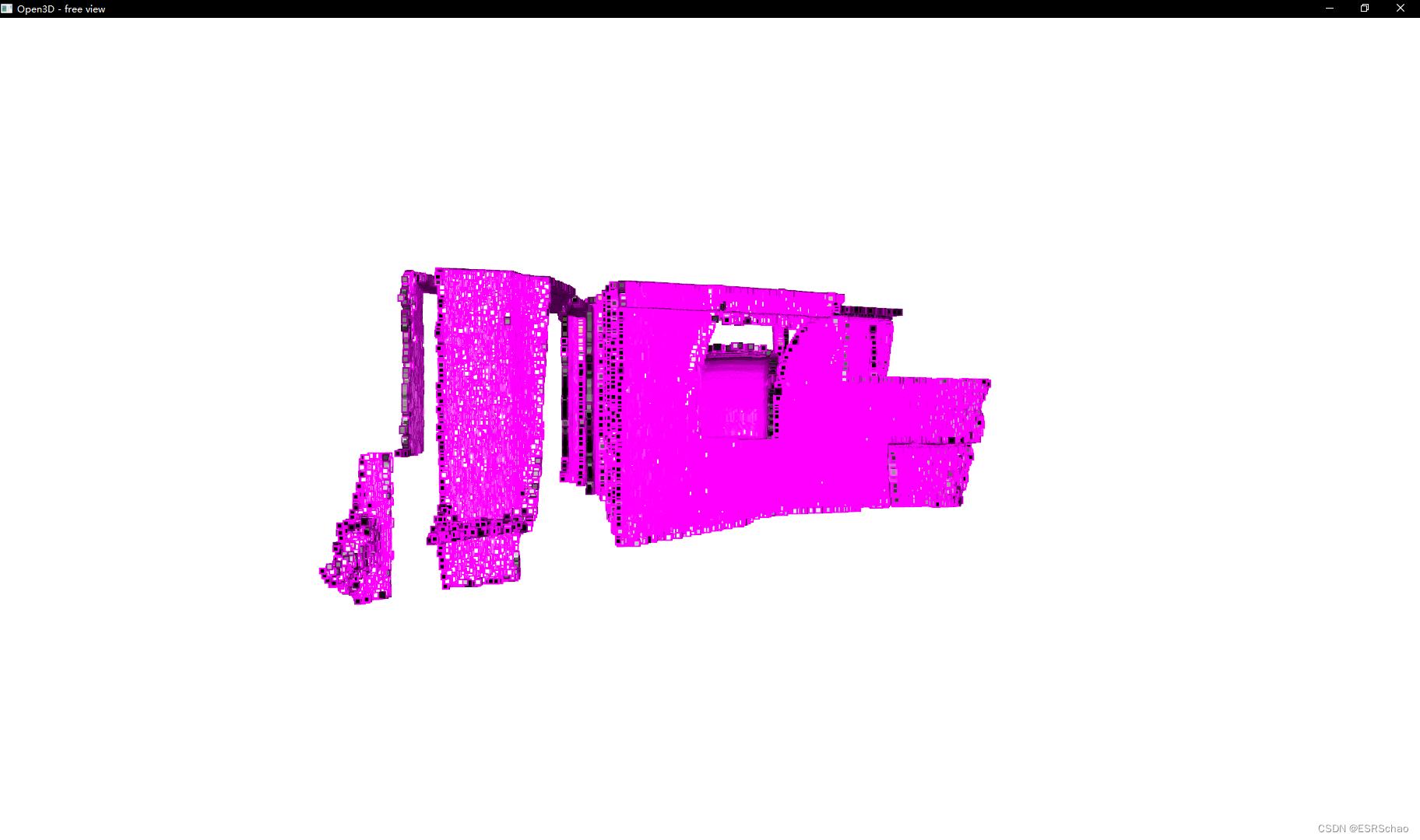
• 输出结果：

ps：这里的输出点云结果相比上面的点云输出结果更加的完善，而且参考的中心坐标点也不一样。

---

5. 鸟瞰图可视化

代码中的鸟瞰图范围可以自行设置。同样，输入的也只需要是.bin文件即可展示其鸟瞰图。

• 参考代码：

import numpy as np
from PIL import Image
import matplotlib.pyplot as plt

# 点云读取:000010.bin这里需要填写文件的位置
kitti_file = r'E:\\Study\\Machine Learning\\Dataset3d\\kitti\\training\\velodyne\\000100.bin'
pointcloud = np.fromfile(file=kitti_file, dtype=np.float32, count=-1).reshape([-1, 4])

# 设置鸟瞰图范围
side_range = (-40, 40)  # 左右距离
# fwd_range = (0, 70.4)  # 后前距离
fwd_range = (-70.4, 70.4)

x_points = pointcloud[:, 0]
y_points = pointcloud[:, 1]
z_points = pointcloud[:, 2]

# 获得区域内的点
f_filt = np.logical_and(x_points > fwd_range[0], x_points < fwd_range[1])
s_filt = np.logical_and(y_points > side_range[0], y_points < side_range[1])
filter = np.logical_and(f_filt, s_filt)
indices = np.argwhere(filter).flatten()
x_points = x_points[indices]
y_points = y_points[indices]
z_points = z_points[indices]

res = 0.1  # 分辨率0.05m
x_img = (-y_points / res).astype(np.int32)
y_img = (-x_points / res).astype(np.int32)
# 调整坐标原点
x_img -= int(np.floor(side_range[0]) / res)
y_img += int(np.floor(fwd_range[1]) / res)
print(x_img.min(), x_img.max(), y_img.min(), x_img.max())

# 填充像素值
height_range = (-2, 0.5)
pixel_value = np.clip(a=z_points, a_max=height_range[1], a_min=height_range[0])


def scale_to_255(a, min, max, dtype=np.uint8):
    return ((a - min) / float(max - min) * 255).astype(dtype)


pixel_value = scale_to_255(pixel_value, height_range[0], height_range[1])

# 创建图像数组
x_max = 1 + int((side_range[1] - side_range[0]) / res)
y_max = 1 + int((fwd_range[1] - fwd_range[0]) / res)
im = np.zeros([y_max, x_max], dtype=np.uint8)
im[y_img, x_img] = pixel_value

# imshow （灰度）
im2 = Image.fromarray(im)
im2.show()

# imshow （彩色）
# plt.imshow(im, cmap="nipy_spectral", vmin=0, vmax=255)
# plt.show()

• 结果展示：

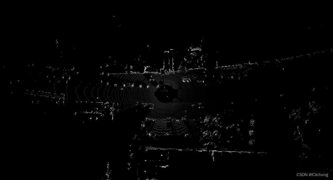
后续的工作会加深对点云数据的理解，整个可视化项目的工程见：KITTI数据集的可视化项目，有需要的朋友可以自行下载。

---

参考资料：

1. KITTI自动驾驶数据集可视化教程

2. kitti数据集在3D目标检测中的入门

3. kitti数据集在3D目标检测中的入门(二)可视化详解

4. kitti_object_vis项目

python如何实现点云可视化交互——Open3D实例教程（获取所选点的信息）保姆级教学

前言

Open3D是目前python中可用的用于 3D 数据处理的现代库，可以对点云、网格等三维数据进行读取、采样、配准、可视化等操作。其中对点云等三维模型进行可视化的功能在Python中显得非常方便。

在通过对官方文档的研究之后作者发现在Open3D的多种可视化函数中出现了返回所选点的信息的命令，将代码跑通后就有了这篇三维物体可视化交互的文章，希望诸位能通过这篇文章获取一些新的思路。

开发环境
python 3.9.12
Open3D 0.15.1
Pycharm 2021.2

点云的可视化

Open3D对于点云的可视化可以采用两种方式，一种是直接用visualization下面的用于绘制几何图形列表的函数draw_geometries来进行显示，另外一种就是使用可视化工具Visualizer来进行显示。
第一种方式简单快捷，但并不能返回所选点的信息，如果读者发现了可以返回值的方法欢迎补充。

1. draw_geometries

Open3D的官方文档中给出了四种不同的draw_geometries

1. draw_geometries —— 用于绘制几何图形列表的函数
2. draw_geometries_with_editing —— 具有编辑功能的用于绘制几何图形列表的函数
3. draw_geometries_with_key_callbacks —— 具有自定义键调用功能的绘制几何图形列表的函数
4. draw_geometries_with_vertex_selection —— 具有顶点选择功能的绘制几何图形列表的函数

除了第一种函数，后三种均可以选取点并在终端里显示选取点的信息，但是并不会返回值，所以我们无法在程序中直接得到所选点的信息。

后三种选取点的可视化效果也不太一样，这边只针对第四种进行说明。

draw_geometries这种方式代码比较简单，平常使用的时候比较方便，感兴趣的可以试着跑跑官方例程：

第一种 draw_geometries

import open3d as o3d
import numpy as np
print("Load a ply point cloud, print it, and render it")
ply_point_cloud = o3d.data.PLYPointCloud()
pcd = o3d.io.read_point_cloud(ply_point_cloud.path)
print(pcd)
print(np.asarray(pcd.points))
o3d.visualization.draw_geometries([pcd],
                                  zoom=0.3412,
                                  front=[0.4257, -0.2125, -0.8795],
                                  lookat=[2.6172, 2.0475, 1.532],
                                  up=[-0.0694, -0.9768, 0.2024])

小提示：在可视化窗口弹出后按H键可以在终端中查看详细的操作菜单

第四种 draw_geometries_with_vertex_selection

import open3d as o3d
import numpy as np
print("Load a ply point cloud, print it, and render it")
ply_point_cloud = o3d.data.PLYPointCloud()
pcd = o3d.io.read_point_cloud(ply_point_cloud.path)
print(pcd)
print(np.asarray(pcd.points))
point = o3d.visualization.draw_geometries_with_key_callbacks([pcd])
print(point)

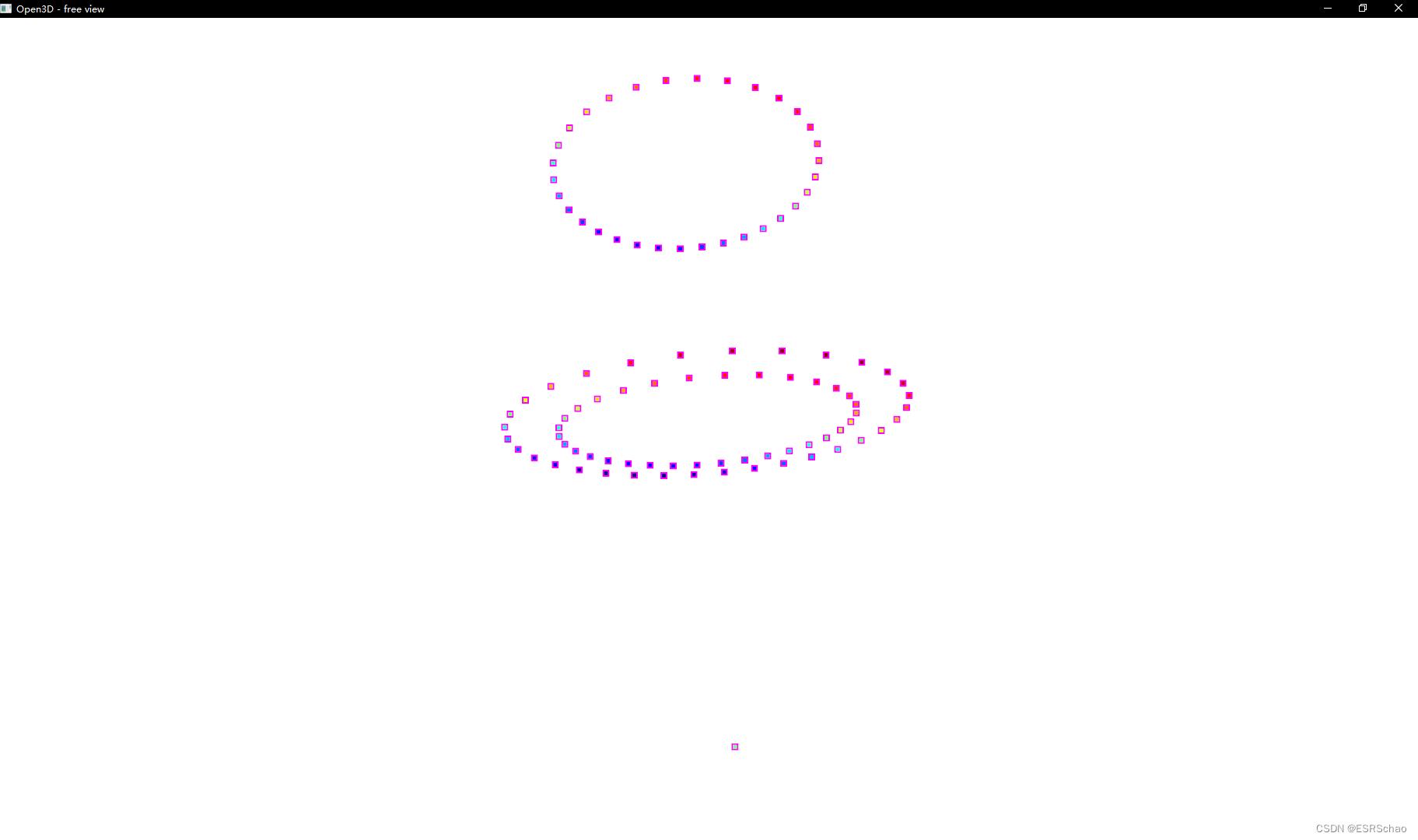
执行代码，可视化窗口跳出

此时在可视化窗口按下Shift键进入点的选择模式：

这时候使用鼠标可以进行顶点的选择，所选点的信息会显示在终端中：
注意：代码中用point来获取返回值信息，而最后打印出来的point是None证明所选点只会在终端中显示出来，并不会返回值

官方文档中也说明了函数是没有返回值的，那么如果想要获得所选点的信息该怎么办呢。这就可以使用另外一种方法了。

2.Visualizer

Open3D的官方文档中也给出了四种不同的Visualizer

1. Visualizer —— 可视化工具主类
2. VisualizerWithEditing —— 具有编辑功能的可视化工具
3. VisualizerWithKeyCallback —— 具有自定义键调用功能的可视化工具
4. VisualizerWithVertexSelection —— 具有顶点选择功能的可视化工具

对于open3d.visualization.Visualizer这种可视化工具，它的基本使用方法可以简单总结为下面几步（作者为了演示简化了各函数参数，感兴趣的读者可以参考官方文档）：

1. 创建vis类
   vis = o3d.visualization.VisualizerWithVertexSelection()
2. 创建可视化窗口
   vis.create_window(window_name=‘Open3D’, width=1920, height=1080, visible=True)
3. 输入点云或者网格数据
   vis.add_geometry(mesh)
4. 激活窗口 此操作会阻塞线程
   vis.run()
5. 清除可视化窗口
   vis.destroy_window()

在可视化过程中也可以通过相关函数进行获得当前视角的RGB图像和深度图等操作，十分方便。

而open3d.visualization.VisualizerWithVertexSelection中增加了一个函数get_picked_points：

get_picked_points(self: open3d.cpu.pybind.visualization.VisualizerWithVertexSelection) → List[open3d::visualization::VisualizerWithVertexSelection::PickedPoint]

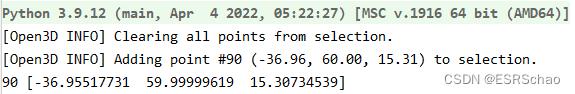
它的描述为Function to get picked points，此函数可以返回在可视化窗口选取点的坐标和索引信息。

下图展示了返回值point的信息，可以看到point列表在选取一个点的情况下有0号点的coord三维位置信息以及index索引信息。

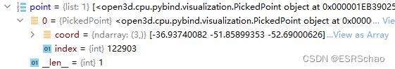
整体的程序如下，用的是我自己的点云模型：

import open3d as o3d
import numpy as np
pcd = o3d.io.read_point_cloud("arrow.ply")
vis = o3d.visualization.VisualizerWithVertexSelection()
vis.create_window(window_name='Open3D', visible=True)
vis.add_geometry(pcd)
vis.run()
point = vis.get_picked_points()
vis.destroy_window()
print(point[0].index, np.asarray(point[0].coord))

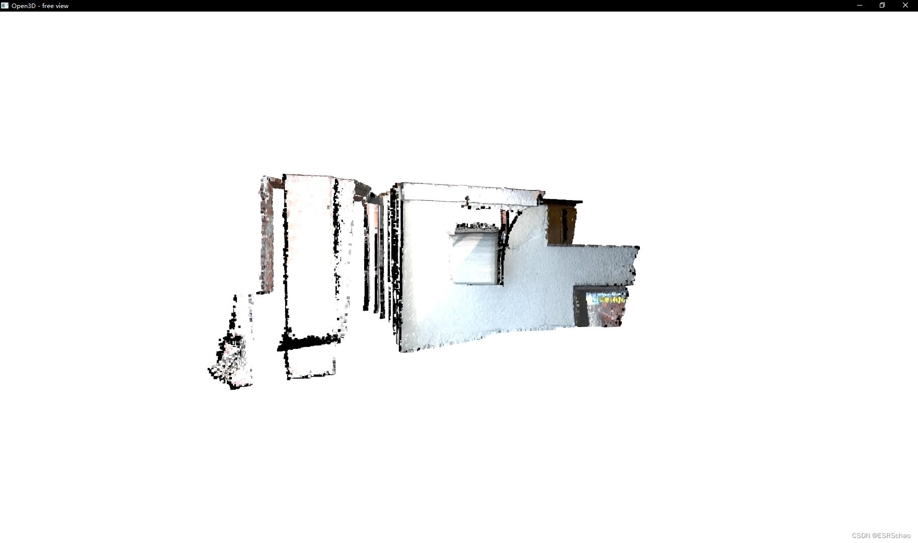
弹出可视化界面

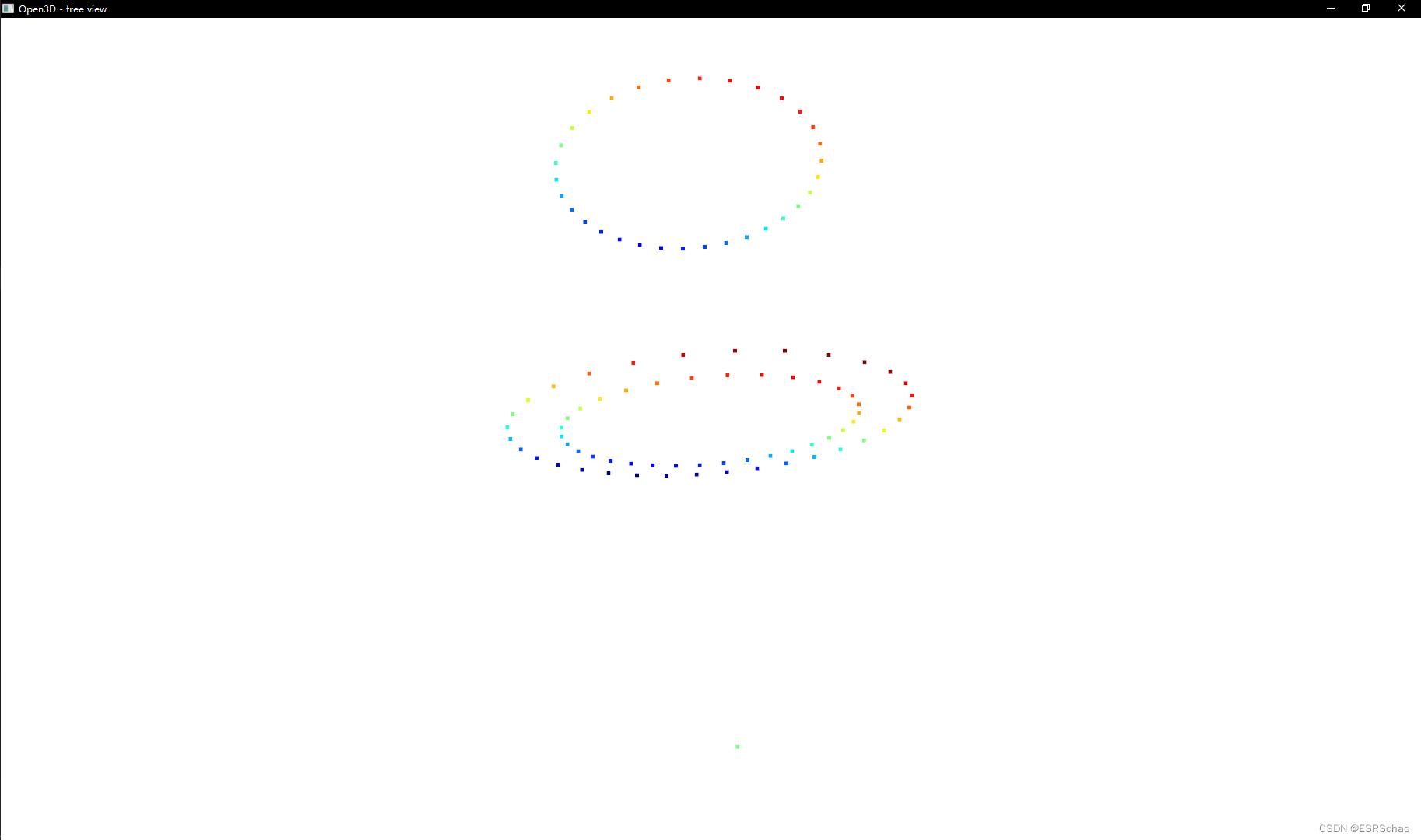
按住Shift键

选取一个或多个点（选中点显示为绿色）

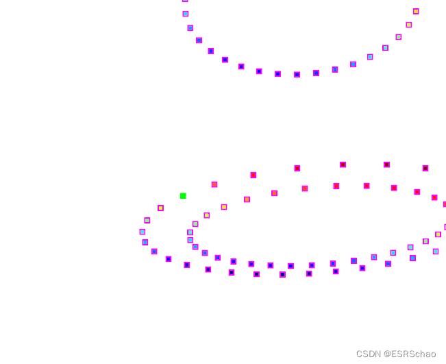
关闭窗口即可获得所选点的信息
而且信息会被储存在point列表中

如此这般就实现了点云的可视化交互，我们可以通过在可视化界面中直接进行选择从而获得一个或者一部分点的信息，进而可以直接在后续的程序中进行处理。

教程书写不易，如果有帮到诸位还请点个赞或者收藏，谢谢大家。