Python曲线拟合(polyfit , curve_fit, interp1d插值)
Posted Forward南
tags:
篇首语:本文由小常识网(cha138.com)小编为大家整理,主要介绍了Python曲线拟合(polyfit , curve_fit, interp1d插值)相关的知识,希望对你有一定的参考价值。
文章目录
np.polyfit 多项式拟合
在python中,Numpy.polyfit()是一个在多项式函数内拟合数据的方法。当最小二乘法的拟合条件很差时,polyfit会发出RankWarning。
对散点进行多项式拟合并打印出拟合函数以及拟合后的图形程序如下
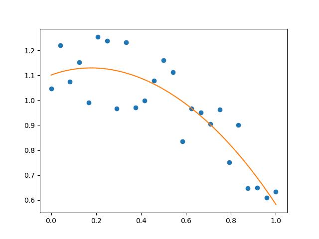
例1
在这个程序中,首先,导入matplotlib和numpy库。设置x、y、p和t的值。然后,使用这个x、y、p和t的值,通过拟合绘制多项式。
import numpy as np
import matplotlib.pyplot as plt

np.random.seed(46)
x = np.linspace(0, 1, 25)
y = np.cos(x) + 0.3 * np.random.rand(25)
p = np.poly1d(np.polyfit(x, y, 4))
t = np.linspace(0, 1, 250)
plt.plot(x, y, 'o', t, p(t), '-')
plt.show()
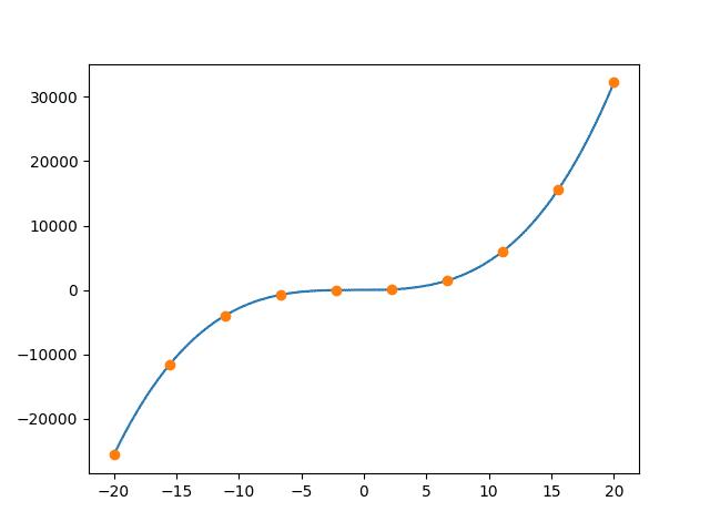
例2
在这个程序中,也是如此,首先,导入matplotlib和numpy库。设置x和y的值。然后,计算多项式并设置x和y的新值。一旦完成,使用函数polyfit()拟合多项式。
import numpy as np
import matplotlib.pyplot as plt

np.random.seed(12)
x = np.linspace(-20, 20, 10)
y = 3.6 * pow(x, 3) + 8.3 * pow(x, 2) + 5.1 * pow(x, 1) + 5
func = np.polyfit(x, y, 4)
xn = np.linspace(-20, 20, 1000)
yn = np.poly1d(func)
plt.plot(xn, yn(xn), x, y, 'o')
plt.show()
curve_fit () 自定义函数拟合
能拟合的函数不止下面这些,只要你写出想要使用的函数的表达式,就可以得到函数的参数!!!
import numpy as np # NumPy https://numpy.org/
import matplotlib.pyplot as plt # Matplotlib https://matplotlib.org/
from scipy.optimize import curve_fit # https://www.scipy.org/
# 三次 - 跟前面所说的poly_fit一个意思
def func_poly_3(x, a, b, c , d):
return a*x*x*x + b*x*x + c*x + d
# 幂函数
def func_power(x, a, b):
return x**a + b
# 指数函数
def func_exp(x, a, b):
return a**x + b
def Hyperb(x, a1, a2, qi):
y = qi / np.power(1 + a1 * a2 * x, 1 / a2)
return y
xdata=[1.0, 1.0185728, 1.0371457, 1.0557185, 1.0742913, 1.0928641, 1.111437, 1.1300098, 1.1485826, 1.1671554, 1.1857283, 1.2043011, 1.2228739, 1.2414467, 1.2600196, 1.2785924, 1.2971652, 1.315738, 1.3343109, 1.3528837, 1.3714565, 1.3900293, 1.4086022, 1.427175, 1.4457478, 1.4643206, 1.4828935, 1.5014663, 1.5200391, 1.5386119, 1.5571848, 1.5757576, 1.5943304, 1.6129032, 1.6314761, 1.6500489, 1.6686217, 1.6871945, 1.7057674, 1.7243402, 1.742913, 1.7614858, 1.7800587, 1.7986315, 1.8172043, 1.8357771, 1.85435, 1.8729228, 1.8914956, 1.9100684, 1.9286413, 1.9472141, 1.9657869, 1.9843597, 2.0029326, 2.0215054, 2.0400782, 2.058651, 2.0772239, 2.0957967, 2.1143695, 2.1329423, 2.1515152, 2.170088, 2.1886608, 2.2072336, 2.2258065, 2.2443793, 2.2629521, 2.2815249, 2.3000978, 2.3186706, 2.3372434, 2.3558162, 2.3743891, 2.3929619, 2.4115347, 2.4301075, 2.4486804, 2.4672532, 2.485826, 2.5043988, 2.5229717, 2.5415445, 2.5601173, 2.5786901, 2.597263, 2.6158358, 2.6344086, 2.6529814, 2.6715543, 2.6901271, 2.7086999, 2.7272727, 2.7458456, 2.7644184, 2.7829912, 2.801564, 2.8201369, 2.8387097, 2.8572825, 2.8758553, 2.8944282, 2.913001, 2.9315738, 2.9501466, 2.9687195, 2.9872923, 3.0058651, 3.0244379, 3.0430108, 3.0615836, 3.0801564, 3.0987292, 3.1173021, 3.1358749, 3.1544477, 3.1730205, 3.1915934, 3.2101662, 3.228739, 3.2473118, 3.2658847, 3.2844575, 3.3030303, 3.3216031, 3.340176, 3.3587488, 3.3773216, 3.3958944, 3.4144673, 3.4330401, 3.4516129, 3.4701857, 3.4887586, 3.5073314, 3.5259042, 3.544477, 3.5630499, 3.5816227, 3.6001955, 3.6187683, 3.6373412, 3.655914, 3.6744868, 3.6930596, 3.7116325, 3.7302053, 3.7487781, 3.7673509, 3.7859238, 3.8044966, 3.8230694, 3.8416422, 3.8602151, 3.8787879, 3.8973607, 3.9159335, 3.9345064, 3.9530792, 3.971652, 3.9902248, 4.0087977, 4.0273705, 4.0459433, 4.0645161, 4.083089, 4.1016618, 4.1202346, 4.1388074, 4.1573803, 4.1759531, 4.1945259, 4.2130987, 4.2316716, 4.2502444, 4.2688172, 4.28739, 4.3059629, 4.3245357, 4.3431085, 4.3616813, 4.3802542, 4.398827, 4.4173998, 4.4359726, 4.4545455, 4.4731183, 4.4916911, 4.5102639, 4.5288368, 4.5474096, 4.5659824, 4.5845552, 4.6031281, 4.6217009, 4.6402737, 4.6588465, 4.6774194, 4.6959922, 4.714565, 4.7331378, 4.7517107, 4.7702835, 4.7888563, 4.8074291, 4.826002, 4.8445748, 4.8631476, 4.8817204, 4.9002933, 4.9188661, 4.9374389, 4.9560117, 4.9745846, 4.9931574, 5.0117302, 5.030303, 5.0488759, 5.0674487, 5.0860215, 5.1045943, 5.1231672, 5.14174, 5.1603128, 5.1788856, 5.1974585, 5.2160313, 5.2346041, 5.2531769, 5.2717498, 5.2903226, 5.3088954, 5.3274682, 5.3460411, 5.3646139, 5.3831867, 5.4017595, 5.4203324, 5.4389052, 5.457478, 5.4760508, 5.4946237, 5.5131965, 5.5317693, 5.5503421, 5.568915, 5.5874878, 5.6060606, 5.6246334, 5.6432063, 5.6617791, 5.6803519, 5.6989247, 5.7174976, 5.7360704, 5.7546432, 5.773216, 5.7917889, 5.8103617, 5.8289345, 5.8475073, 5.8660802, 5.884653, 5.9032258, 5.9217986, 5.9403715, 5.9589443, 5.9775171, 5.9960899, 6.0146628, 6.0332356, 6.0518084, 6.0703812, 6.0889541, 6.1075269, 6.1260997, 6.1446725, 6.1632454, 6.1818182, 6.200391, 6.2189638, 6.2375367, 6.2561095, 6.2746823, 6.2932551, 6.311828, 6.3304008, 6.3489736, 6.3675464, 6.3861193, 6.4046921, 6.4232649, 6.4418377, 6.4604106, 6.4789834, 6.4975562, 6.516129, 6.5347019, 6.5532747, 6.5718475, 6.5904203, 6.6089932, 6.627566, 6.6461388, 6.6647116, 6.6832845, 6.7018573, 6.7204301, 6.7390029, 6.7575758, 6.7761486, 6.7947214, 6.8132942, 6.8318671, 6.8504399, 6.8690127, 6.8875855, 6.9061584, 6.9247312, 6.943304, 6.9618768, 6.9804497, 6.9990225, 7.0175953, 7.0361681, 7.054741, 7.0733138, 7.0918866, 7.1104594, 7.1290323, 7.1476051, 7.1661779, 7.1847507, 7.2033236, 7.2218964, 7.2404692, 7.259042, 7.2776149, 7.2961877, 7.3147605, 7.3333333, 7.3519062, 7.370479, 7.3890518, 7.4076246, 7.4261975, 7.4447703, 7.4633431, 7.4819159, 7.5004888, 7.5190616, 7.5376344, 7.5562072, 7.5747801, 7.5933529, 7.6119257, 7.6304985, 7.6490714, 7.6676442, 7.686217, 7.7047898, 7.7233627, 7.7419355, 7.7605083, 7.7790811, 7.797654, 7.8162268, 7.8347996, 7.8533724, 7.8719453, 7.8905181, 7.9090909, 7.9276637, 7.9462366, 7.9648094, 7.9833822, 8.001955, 8.0205279, 8.0391007, 8.0576735, 8.0762463, 8.0948192, 8.113392, 8.1319648, 8.1505376, 8.1691105, 8.1876833, 8.2062561, 8.2248289, 8.2434018, 8.2619746, 8.2805474, 8.2991202, 8.3176931, 8.3362659, 8.3548387, 8.3734115, 8.3919844, 8.4105572, 8.42913, 8.4477028, 8.4662757, 8.4848485, 8.5034213, 8.5219941, 8.540567, 8.5591398, 8.5777126, 8.5962854, 8.6148583, 8.6334311, 8.6520039, 8.6705767, 8.6891496, 8.7077224, 8.7262952, 8.744868, 8.7634409, 8.7820137, 8.8005865, 8.8191593, 8.8377322, 8.856305, 8.8748778, 8.8934506, 8.9120235, 8.9305963, 8.9491691, 8.9677419, 8.9863148, 9.0048876, 9.0234604, 9.0420332, 9.0606061, 9.0791789, 9.0977517, 9.1163245, 9.1348974, 9.1534702, 9.172043, 9.1906158, 9.2091887, 9.2277615, 9.2463343, 9.2649071, 9.28348, 9.3020528, 9.3206256, 9.3391984, 9.3577713, 9.3763441, 9.3949169, 9.4134897, 9.4320626, 9.4506354, 9.4692082, 9.487781, 9.5063539, 9.5249267, 9.5434995, 9.5620723, 9.5806452, 9.599218, 9.6177908, 9.6363636, 9.6549365, 9.6735093, 9.6920821, 9.7106549, 9.7292278, 9.7478006, 9.7663734, 9.7849462, 9.8035191, 9.8220919, 9.8406647, 9.8592375, 9.8778104, 9.8963832, 9.914956, 9.9335288, 9.9521017, 9.9706745, 9.9892473, 10.00782, 10.026393, 10.044966, 10.063539, 10.082111, 10.100684, 10.119257, 10.13783, 10.156403, 10.174976, 10.193548, 10.212121, 10.230694, 10.249267, 10.26784, 10.286413, 10.304985, 10.323558, 10.342131, 10.360704, 10.379277, 10.397849, 10.416422, 10.434995, 10.453568, 10.472141, 10.490714, 10.5, 10.509286, 10.527859, 10.546432, 10.565005, 10.583578, 10.602151, 10.620723, 10.639296, 10.657869, 10.676442, 10.695015, 10.713587, 10.73216, 10.750733, 10.769306, 10.787879, 10.806452, 10.825024, 10.843597, 10.86217, 10.880743, 10.899316, 10.917889, 10.936461, 10.955034, 10.973607, 10.99218, 11.010753, 11.029326, 11.047898, 11.066471, 11.085044, 11.103617, 11.12219, 11.140762, 11.159335, 11.177908, 11.196481, 11.215054, 11.233627, 11.252199, 11.270772, 11.289345, 11.307918, 11.326491, 11.345064, 11.363636, 11.382209, 11.400782, 11.419355, 11.437928, 11.4565, 11.475073, 11.493646, 11.512219, 11.530792, 11.549365, 11.567937, 11.58651, 11.605083, 11.623656, 11.642229, 11.660802, 11.679374, 11.697947, 11.71652, 11.735093, 11.753666, 11.772239, 11.790811, 11.809384, 11.827957, 11.84653, 11.865103, 11.883675, 11.902248, 11.920821, 11.939394, 11.957967, 11.97654, 11.995112, 12.013685, 12.032258, 12.050831, 12.069404, 12.087977, 12.106549, 12.125122, 12.143695, 12.162268, 12.180841, 12.199413, 12.217986, 12.236559, 12.255132, 12.273705, 12.292278, 12.31085, 12.329423, 12.347996, 12.366569, 12.385142, 12.403715, 12.422287, 12.44086, 12.459433, 12.478006, 12.496579, 12.515152, 12.533724, 12.552297, 12.57087, 12.589443, 12.608016, 12.626588, 12.645161, 12.663734, 12.682307, 12.70088, 12.719453, 12.738025, 12.756598, 12.775171, 12.793744, 12.812317, 12.83089, 12.849462, 12.868035, 12.886608, 12.905181, 12.923754, 12.942326, 12.960899, 12.979472Python做曲线拟合(一元多项式拟合及任意函数拟合)
目录
1. 一元多项式拟合
使用方法 np.polyfit(x, y, deg)
polyfig 使用的是最小二乘法,用于拟合一元多项式函数。
参数说明: x 就是x坐标,y 就是y坐标,deg 为拟合多项式的次数。
实例:
根据 ti yi 两个列表来得到 一元二次多项式拟合函数 (deg为2)
import matplotlib.pyplot as plt
import numpy as np
import pylab as mpl
ti = [1, 1.5, 2, 2.5, 3, 3.5, 4, 4.5, 5, 5.5, 6, 6.5, 7, 7.5, 8]
yi = [33.40, 79.50, 122.65, 159.05, 189.15, 214.15, 238.65, 252.2, 267.55, 280.50, 296.65, 301.65, 310.4, 318.15, 325.15]
z1 = np.polyfit(ti, yi, 2)
print(z1)
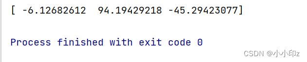
输出结果:
分别是二次多项式的 3 个系数,y = ax^2 + bx + c
2. 任意函数拟合
使用 curve_fit() 方法
curve_fit() 使用是非线性最小二乘法将函数进行拟合,适用范围:多元、任意函数
scipy.optimize.curve_fit(f,xdata,ydata,p0 = None)
常用参数说明:
f: 模型函数f(x,…)。它必须将自变量作为第一个参数,其余你需要求的参数都放后面
xdata: 数组对象,测量数据的自变量。
ydata: 数组对象,因变量。
p0:参数的初始猜测(长度 N),如果为None,则初始值为1(如果可以使用自省来确定函数的参数数量,否则会引发 ValueError)。
返回值:
popt: 数组,参数的最佳值,以使的平方残差之和最小。f(xdata, *popt) - ydata
pcov: 二维阵列,popt的估计协方差。对角线提供参数估计的方差。
实例:
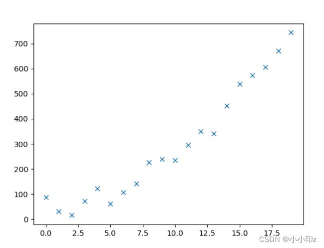
(1)初始化 x 和 y 数据集
x 为 0~19(包括0和19),y=2x^2 + (二十个0~100范围内的随机数)
import numpy as np
x = np.arange(0,20)
y = 2 * x ** 2 + np.random.randint(0, 100, 20)
#z = 2 * x ** 2 + np.random.randint(0, 100, (1,20))[0]
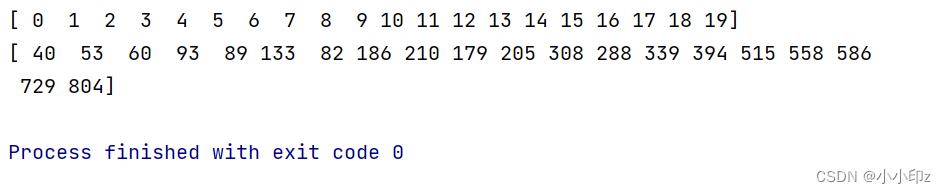
如图为生成 x 列表和 y 列表的值(具有随机性):
补充一下 np.random.randint()用法:
numpy.random.randint(low, high=None, size=None, dtype=int)
参数说明:
1. low: int 生成的数值的最小值(包含),默认为0,可省略。
2. high: int 生成的数值的最大值(不包含)。
3. size: int or tuple of ints 随机数的尺寸, 默认是返回单个,输入 20 返回 20个,输入 (3,4) 返回的是一个 3*4 的二维数组。(可选)。
4. dtype:想要输出的结果类型。默认值为int。(可选,一般用不上)。
(2)建立自定义函数
定义函数 y=ax^2
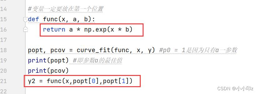
#变量一定要放在第一个位置
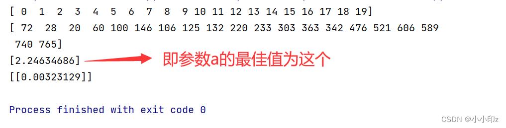
def func(x, a):
return a*x**2
popt, pcov = curve_fit(func, x, y, p0=1) #p0 = 1是因为只有a一参数
print(popt) #即参数a的最佳值
print(pcov)
输出结果:
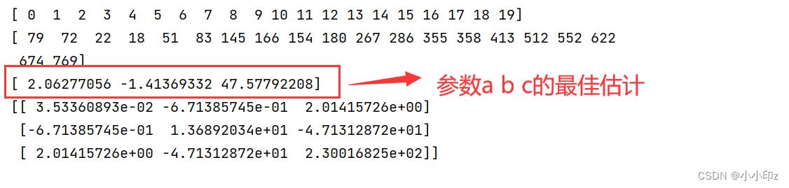
定义函数 y=2x^2+bx+c
#变量一定要放在第一个位置
def func(x, a, b, c):
return a*x**2 + b*x + c
popt, pcov = curve_fit(func, x, y) #p0 = 1是因为只有a一参数
print(popt) #即参数a的最佳值
print(pcov)
输出结果:
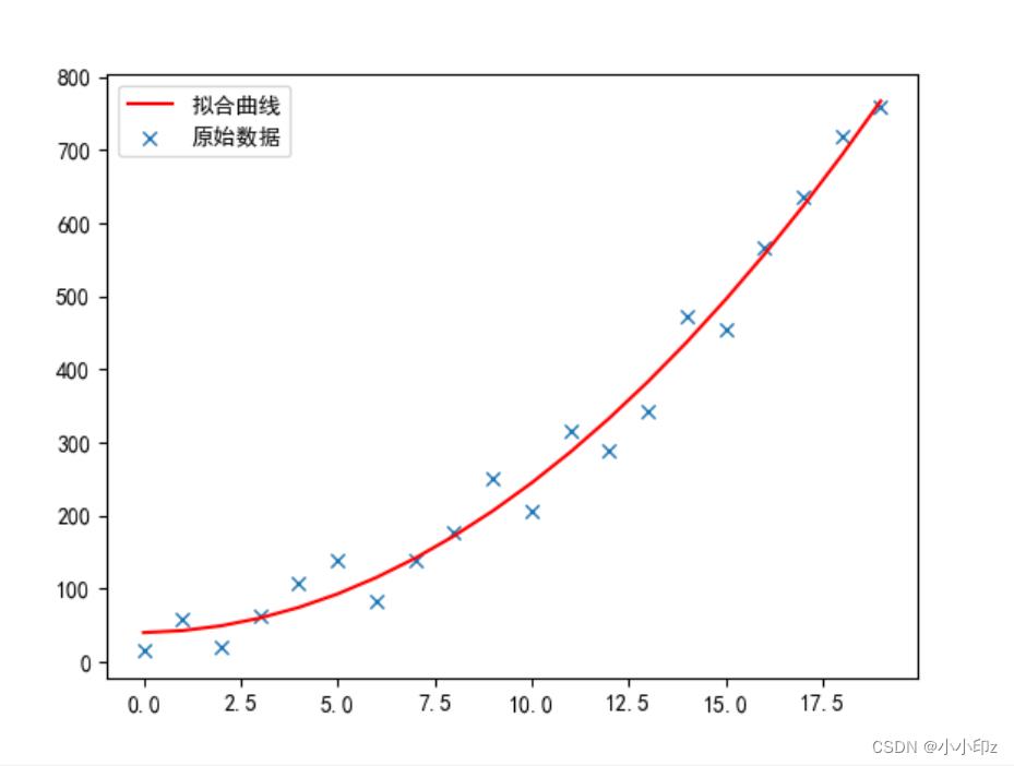
(3)使用自定义的函数生成拟合函数绘图
对第二个拟合函数绘图:
完整代码:
注意:在画图是可能会出现坐标中文乱码的问题,需要加入以下几行:
import pylab as mpl
mpl.rcParams['font.sans-serif'] = ['SimHei'] # 解决中文不显示问题 plt.rcParams['axes.unicode_minus']=False #解决负数坐标显示问题
import numpy as np
import matplotlib.pyplot as plt
from scipy.optimize import curve_fit
import pylab as mpl
mpl.rcParams['font.sans-serif'] = ['SimHei'] # 解决中文不显示问题
plt.rcParams['axes.unicode_minus']=False #解决负数坐标显示问题
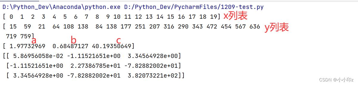
x = np.arange(0,20)
y = 2 * x ** 2 + np.random.randint(0, 100, 20)
z = 2 * x ** 2 + np.random.randint(0, 100, (1,20))[0]
print(x)
print(y)
#变量一定要放在第一个位置
def func(x, a, b, c):
return a*x**2 + b*x + c
popt, pcov = curve_fit(func, x, y) #p0 = 1是因为只有a一参数
print(popt) #即参数a的最佳值
print(pcov)
#popt[0],popt[1],popt[2]分别代表参数a b c
y2 = func(x,popt[0],popt[1],popt[2])
plt.scatter(x, y, marker='x',lw=1,label='原始数据')
plt.plot(x,y2,c='r',label='拟合曲线')
plt.legend() # 显示label
plt.show()
运行结果:
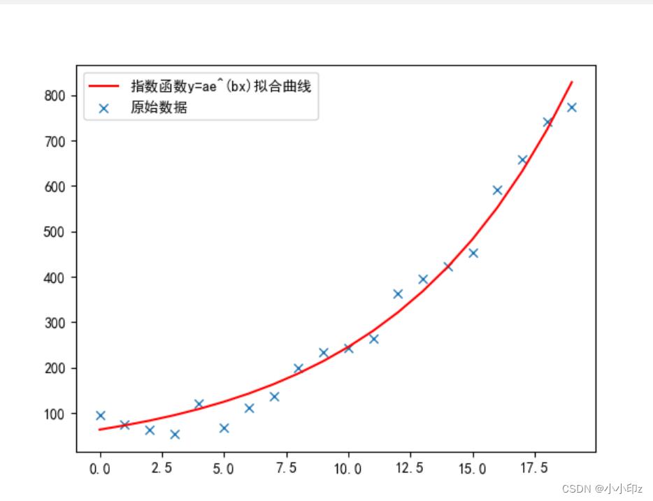
使用指数函数:
y = ae^(bx)
绘图效果:
以上是关于Python曲线拟合(polyfit , curve_fit, interp1d插值)的主要内容,如果未能解决你的问题,请参考以下文章