机器学习1 线性回归（Linear Regression）

Posted 2022-06-23 拉风小宇

tags:

篇首语：本文由小常识网(cha138.com)小编为大家整理，主要介绍了机器学习1 线性回归（Linear Regression）相关的知识，希望对你有一定的参考价值。

立个flag，本人从今天正式开始学习机器学习（Machine Learning）
选取的第一门课还是吴恩达（Andrew Ng）的斯坦福大学公开课：机器学习课程，我打算从作业入手，结合课程进行学习，预计一共分为8篇，这是第一篇

单变量线性回归

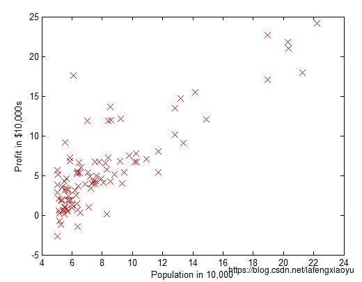
给定是数据集包括97个数组，其中第一个表示人口数，第二个表示盈利数，我们希望得到两者之间的线性表达关系。下图是将点在坐标轴中绘制出来

%% ======================= Part 2: Plotting =======================
fprintf('Plotting Data ...\\n')
data = load('ex1data1.txt');
X = data(:, 1); y = data(:, 2);
m = length(y); % number of training examples

% Plot Data
% Note: You have to complete the code in plotData.m
plotData(X, y);

线性回归的目的是最小化损失函数

梯度下降

损失函数为

J(θ)=12∑i=1m(hθ(x(i))−y(i))2 J ( θ ) = 1 2 ∑ i = 1 m ( h θ ( x ( i ) ) − y ( i ) ) 2 $J(\\theta)=\\frac12\\sum_i=1^m(h_\\theta(x^(i))-y^(i))^2$
这里我们的假设为

hθ h θ $h_\\theta$ 是下面的线性模型

hθ(x)=θTx=θ0+θ1x1 h θ ( x ) = θ T x = θ 0 + θ 1 x 1 $h_\\theta(x)=\\theta^Tx=\\theta_0+\\theta_1x_1$
根据批梯度下降（batch gradient descent）

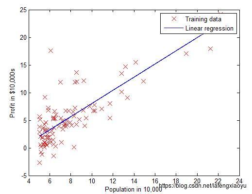
θj:=θj+α∑i=1m(y(i)−hθ(x(i)))x(i)j θ j := θ j + α ∑ i = 1 m ( y ( i ) − h θ ( x ( i ) ) ) x j ( i ) $\\theta_j:=\\theta_j+\\alpha\\sum_i=1^m(y^(i)-h_\\theta(x^(i)))x_j^(i)$
或者根据随机梯度下降方法（stochastic gradient descent）求得

θ θ $\\theta$ 的值，并且绘制出图

%% =================== Part 3: Gradient descent ===================
fprintf('Running Gradient Descent ...\\n')

X = [ones(m, 1), data(:,1)]; % Add a column of ones to x
theta = zeros(2, 1); % initialize fitting parameters

% Some gradient descent settings
iterations = 1500;
alpha = 0.01;

% compute and display initial cost
computeCost(X, y, theta)

% run gradient descent
theta = gradientDescent(X, y, theta, alpha, iterations);

% print theta to screen
fprintf('Theta found by gradient descent: ');
fprintf('%f %f \\n', theta(1), theta(2));

% Plot the linear fit
hold on; % keep previous plot visible
plot(X(:,2), X*theta, '-')
legend('Training data', 'Linear regression')
hold off % don't overlay any more plots on this figure

其中计算代价函数和计算梯度下降分别为

function J = computeCost(X, y, theta)
%COMPUTECOST Compute cost for linear regression
%   J = COMPUTECOST(X, y, theta) computes the cost of using theta as the
%   parameter for linear regression to fit the data points in X and y

% Initialize some useful values
m = length(y); % number of training examples

% You need to return the following variables correctly 
J = 0;

% ====================== YOUR CODE HERE ======================
% Instructions: Compute the cost of a particular choice of theta
%               You should set J to the cost.
h = X * theta;
Jtemp= (h - y).^2;

J = sum(Jtemp) * (1/(2*m));

% =========================================================================

end

和

function [theta, J_history] = gradientDescent(X, y, theta, alpha, num_iters)
%GRADIENTDESCENT Performs gradient descent to learn theta
%   theta = GRADIENTDESENT(X, y, theta, alpha, num_iters) updates theta by 
%   taking num_iters gradient steps with learning rate alpha

% Initialize some useful values
m = length(y); % number of training examples
J_history = zeros(num_iters, 1);

for iter = 1:num_iters

    % ====================== YOUR CODE HERE ======================
    % Instructions: Perform a single gradient step on the parameter vector
    %               theta. 
    %
    % Hint: While debugging, it can be useful to print out the values
    %       of the cost function (computeCost) and gradient here.
    %
    h = X * theta;

    hmy = (h-y) .* X(:,1);
    hmyx =(h-y) .* X(:,2);
    val = sum(hmy) * (1/m);
    val1 = sum(hmyx) * (1/m);
    temp1 = theta(1) - (alpha * val) ;
    temp2 =  theta(2) - (alpha * val1) ;
    theta(1) = temp1;
    theta(2) = temp2;

    %delta = [val;val1];
    %theta = theta - delta .* alpha; 
    %computeCost(X, y, theta)
    %theta
    % ============================================================

    % Save the cost J in every iteration    
    J_history(iter) = computeCost(X, y, theta);

end

end

可视化 $J(\\theta)$

在三维空间画出 $J(\\theta)$ 关于 $\\theta_0$ 和 $theta_1$ 的图并且在图中显示出变化情况如下图所示

三维图	等高线图

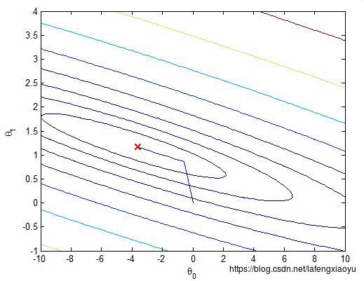代码如下

%% ============= Part 4: Visualizing J(theta_0, theta_1) =============
fprintf('Visualizing J(theta_0, theta_1) ...\\n')

% Grid over which we will calculate J
theta0_vals = linspace(-10, 10, 100);
theta1_vals = linspace(-1, 4, 100);

% initialize J_vals to a matrix of 0's
J_vals = zeros(length(theta0_vals), length(theta1_vals));

% Fill out J_vals
for i = 1:length(theta0_vals)
    for j = 1:length(theta1_vals)
      t = [theta0_vals(i); theta1_vals(j)];    
      J_vals(i,j) = computeCost(X, y, t);
    end
end


% Because of the way meshgrids work in the surf command, we need to 
% transpose J_vals before calling surf, or else the axes will be flipped
J_vals = J_vals';
% Surface plot
figure;
surf(theta0_vals, theta1_vals, J_vals)
xlabel('\\theta_0'); ylabel('\\theta_1');

% Contour plot
figure;
% Plot J_vals as 15 contours spaced logarithmically between 0.01 and 100
contour(theta0_vals, theta1_vals, J_vals, logspace(-2, 3, 20))
xlabel('\\theta_0'); ylabel('\\theta_1');
hold on;
plot(theta(1), theta(2), 'rx', 'MarkerSize', 10, 'LineWidth', 2);

多变量线性回归

这里举的例子是波特兰当地的房价与两个因素之间的关系，分别是房间的大小以及卧室的数目。

特征数据归一化处理

首先我们需要进行标准化处理，因为面积大约是房间数的一千倍，如果直接按照数字处理显然会有很大误差，因此我们这里需要做正规化处理，求出两个特征的平均值和方差，然后再用每个数据减去平均值后在除以标准差，这样的数据符合标准正态分布。
归一化处理的函数如下

function [X_norm, mu, sigma] = featureNormalize(X)
%FEATURENORMALIZE Normalizes the features in X 
%   FEATURENORMALIZE(X) returns a normalized version of X where
%   the mean value of each feature is 0 and the standard deviation
%   is 1. This is often a good preprocessing step to do when
%   working with learning algorithms.

% You need to set these values correctly
X_norm = X;
mu = zeros(1, size(X, 2));
sigma = zeros(1, size(X, 2));

% ====================== YOUR CODE HERE ======================
% Instructions: First, for each feature dimension, compute the mean
%               of the feature and subtract it from the dataset,
%               storing the mean value in mu. Next, compute the 
%               standard deviation of each feature and divide
%               each feature by it's standard deviation, storing
%               the standard deviation in sigma. 
%
%               Note that X is a matrix where each column is a 
%               feature and each row is an example. You need 
%               to perform the normalization separately for 
%               each feature. 
%
% Hint: You might find the 'mean' and 'std' functions useful.
%       
mu = mean(X)
sigma = std(X)

for i = 1:size(X,2)
    X_norm(:,i) = ((X(:,i) - mu(:,i))/sigma(:,i));
end

% ============================================================

end

梯度下降

与之前单变量的做法一样，只不过 $\\theta$ 的数目变了而已
并且在多变量情况下，代价函数 $J(\\theta)$ 可以表示为如下的向量形式

J(θ)=12m(Xθ−y→)T(Xθ−y→) J ( θ ) = 1 2 m ( X θ − y → ) T ( X θ − y → ) $J(\\theta)=\\frac12m(X\\theta-\\overrightarrowy)^T(X\\theta-\\overrightarrowy)$
其中

X=⎡⎣⎢⎢⎢⎢⎢−(x(1))T−机器学习1 线性回归（Linear Regression）

机器学习------- 线性回归（Linear regression ）

机器学习:局部加权线性回归(Locally Weighted Linear Regression)

机器学习---线性回归（Machine Learning Linear Regression）

coursera 机器学习 linear regression 线性回归的小项目

机器学习七--回归--多元线性回归Multiple Linear Regression

机器学习1 线性回归（Linear Regression）

单变量线性回归

梯度下降

可视化 J(θ) J ( θ ) J(\\theta)

多变量线性回归

特征数据归一化处理

梯度下降

可视化 $J(\\theta)$