基于 Tensorflow 2.x 实现多层卷积神经网络，实践 Fashion MNIST 服装图像识别

Posted 2023-02-17 小毕超

一、 Fashion MNIST 服装数据集

Fashion MNIST 数据集，该数据集包含 10 个类别的 70000 个灰度图像。大小统一是 28x28的长宽，其中 60000 张作为训练数据，10000张作为测试数据，该数据集已被封装在了 tf.keras.datasets 工具包下，数据如图所示：

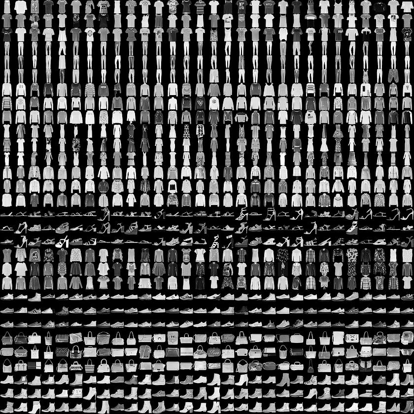
Fashion MNIST 数据集更多样化，比常规 MNIST 更具挑战性。标签是整数数组，介于 0 到 9 之间。这些标签对应于图像所代表的服装类：

标签	分类
0	T恤/上衣
1	裤子
2	套头衫
3	连衣裙
4	外套
5	凉鞋
6	衬衫
7	运动鞋
8	包
9	短靴

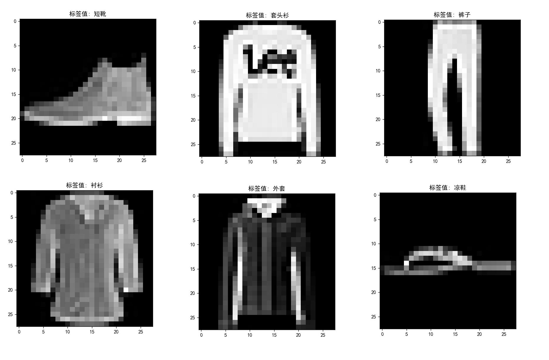
可以通过下面程序对该数据进行可视化预览：

import tensorflow as tf
import matplotlib.pyplot as plt

keras = tf.keras
fashion_mnist = tf.keras.datasets.fashion_mnist
plt.rcParams['font.sans-serif'] = ['SimHei']

classify = 
    0: 'T恤/上衣',
    1: '裤子',
    2: '套头衫',
    3: '连衣裙',
    4: '外套',
    5: '凉鞋',
    6: '衬衫',
    7: '运动鞋',
    8: '包',
    9: '短靴'


# 加载 fashion_mnist 数据集
(x_train, y_train), (x_test, y_test) = fashion_mnist.load_data()

print(x_train.shape)
print(y_train.shape)

for i in range(10):
    image = x_test[i]/255.0
    label = y_test[i]
    plt.imshow(image, cmap=plt.cm.gray)
    plt.title(label=('标签值: ' + str(classify[label])))
    plt.show()

二、搭建多层卷积神经网络模型

本文基于 Tensorflow 2.x 构建多层卷积神经网络，在 Tensorflow 2.x 中官方更推荐的上层API工具为 Keras ，本文也是使用 Keras 进行实验测试。

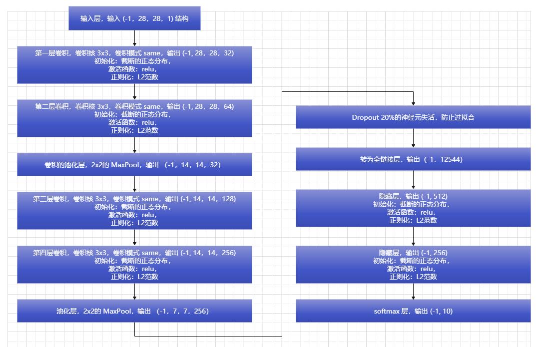
设计模型结构如下所示：

通过 Keras 建立模型结构，具体的解释都写在了注释中：

import tensorflow as tf

keras = tf.keras
fashion_mnist = tf.keras.datasets.fashion_mnist

# 定义模型类
class mnistModel():
    # 初始化结构
    def __init__(self, checkpoint_path, log_path, model_path):
        # checkpoint 权重保存地址
        self.checkpoint_path = checkpoint_path
        # 训练日志保存地址
        self.log_path = log_path
        # 训练模型保存地址：
        self.model_path = model_path
        # 初始化模型结构
        self.model = tf.keras.models.Sequential([
            # 输入层，第一层卷积 ，卷积核 3x3 ，输出 (None, 28, 28, 32)，卷积模式 same
            keras.layers.Conv2D(32, (3, 3),
                                kernel_initializer=keras.initializers.truncated_normal(stddev=0.05),
                                activation=tf.nn.relu,
                                kernel_regularizer=keras.regularizers.l2(0.001),
                                padding='same',
                                input_shape=(28, 28, 1)),
            # 输入层，第二层卷积 ，卷积核 3x3 ，输出 (None, 28, 28, 64)，卷积模式 same
            keras.layers.Conv2D(32, (3, 3),
                                kernel_initializer=keras.initializers.truncated_normal(stddev=0.05),
                                activation=tf.nn.relu,
                                kernel_regularizer=keras.regularizers.l2(0.001),
                                padding='same',
                                input_shape=(28, 28, 1)),
            # 池化层，2x2 MaxPool，输出 (None, 14, 14, 64)
            keras.layers.MaxPooling2D(2, 2),

            # 第三层卷积 ，卷积核 3x3 ，输出 (None, 14, 14, 128) ，卷积模式 same
            keras.layers.Conv2D(64, (3, 3),
                                kernel_initializer=keras.initializers.truncated_normal(stddev=0.05),
                                activation=tf.nn.relu,
                                kernel_regularizer=keras.regularizers.l2(0.001),
                                padding='same'),
            # 第四层卷积 ，卷积核 3x3 ，输出 (None, 14, 14, 256) ，卷积模式 same
            keras.layers.Conv2D(64, (3, 3),
                                kernel_initializer=keras.initializers.truncated_normal(stddev=0.05),
                                activation=tf.nn.relu,
                                kernel_regularizer=keras.regularizers.l2(0.001),
                                padding='same'),
            # 池化层，2x2 MaxPool，输出 (None, 7, 7, 256)
            keras.layers.MaxPooling2D(2, 2),
            # Dropout 随机失活，防止过拟合，输出 (None, 7, 7, 256)
            keras.layers.Dropout(0.2),
            # 转为全链接层，输出 (None, 12544)
            keras.layers.Flatten(),
            # 第一层全链接层，输出 (None, 512)
            keras.layers.Dense(512,
                               kernel_initializer=keras.initializers.truncated_normal(stddev=0.05),
                               kernel_regularizer=keras.regularizers.l2(0.001),
                               activation=tf.nn.relu),
            # 第二层全链接层，输出 (None, 256)
            keras.layers.Dense(256,
                               kernel_initializer=keras.initializers.truncated_normal(stddev=0.05),
                               kernel_regularizer=keras.regularizers.l2(0.001),
                               activation=tf.nn.relu),
            # softmax 层，输出 (None, 10)
            keras.layers.Dense(10, activation=tf.nn.softmax)
        ])

    # 编译模型
    def compile(self):
        # 输出模型摘要
        self.model.summary()
        # 定义训练模式
        self.model.compile(optimizer='adam',
                           loss='sparse_categorical_crossentropy',
                           metrics=['accuracy'])

    # 训练模型
    def train(self, x_train, y_train):
        # tensorboard 训练日志收集
        tensorboard = keras.callbacks.TensorBoard(log_dir=self.log_path)

        # 训练过程保存 Checkpoint 权重，防止意外停止后可以继续训练
        model_checkpoint = keras.callbacks.ModelCheckpoint(self.checkpoint_path,  # 保存模型的路径
                                                           monitor='val_loss',  # 被监测的数据。
                                                           verbose=0,  # 详细信息模式，0 或者 1
                                                           save_best_only=True,  # 如果 True， 被监测数据的最佳模型就不会被覆盖
                                                           save_weights_only=True,
                                                           # 如果 True，那么只有模型的权重会被保存 (model.save_weights(filepath))，否则的话，整个模型会被保存,(model.save(filepath))
                                                           mode='auto',
                                                           # auto, min, max的其中之一。 如果 save_best_only=True，那么是否覆盖保存文件的决定就取决于被监测数据的最大或者最小值。 对于 val_acc，模式就会是 max，而对于 val_loss，模式就需要是 min，等等。 在 auto模式中，方向会自动从被监测的数据的名字中判断出来。
                                                           period=3  # 每3个epoch保存一次权重
                                                           )
        # 填充数据，迭代训练
        self.model.fit(
            x_train,  # 训练集
            y_train,  # 训练集的标签
            validation_split=0.2,  # 验证集的比例
            epochs=30,  # 迭代周期
            batch_size=30,  # 一批次输入的大小
            verbose=2,  # 训练过程的日志信息显示，一个epoch输出一行记录
            callbacks=[tensorboard, model_checkpoint]
        )
        # 保存训练模型
        self.model.save(self.model_path)

    def evaluate(self, x_test, y_test):
        # 评估模型
        test_loss, test_acc = self.model.evaluate(x_test, y_test)
        return test_loss, test_acc

上面优化器使用的 adam，loss 为 sparse_categorical_crossentropy，一共训练 30 个周期，每个 batch 30 张图片，验证集的比例为 20%，并且每三个周期保存一次权重，防止意外停止后继续训练，最后保存了 h5 的训练模型，方便后面进行测试预测效果。

下面开始训练模型：

import tensorflow as tf

keras = tf.keras
fashion_mnist = tf.keras.datasets.fashion_mnist

def main():
    # 加载数据集
    (x_train, y_train), (x_test, y_test) = fashion_mnist.load_data()
    # 修改shape 数据归一化
    x_train, x_test = x_train.reshape(60000, 28, 28, 1) / 255.0, \\
                      x_test.reshape(10000, 28, 28, 1) / 255.0

    checkpoint_path = './checkout/'
    log_path = './log'
    model_path = './model/model.h5'

    # 构建模型
    model = mnistModel(checkpoint_path, log_path, model_path)
    # 编译模型
    model.compile()
    # 训练模型
    model.train(x_train, y_train)
    # 评估模型
    test_loss, test_acc = model.evaluate(x_test, y_test)
    print(test_loss, test_acc)

if __name__ == '__main__':
    main()

运行后可以看到打印的网络结构：

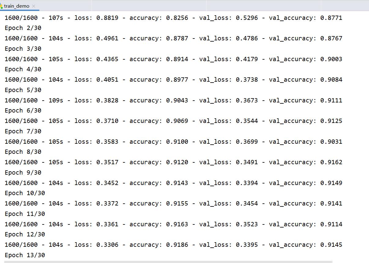
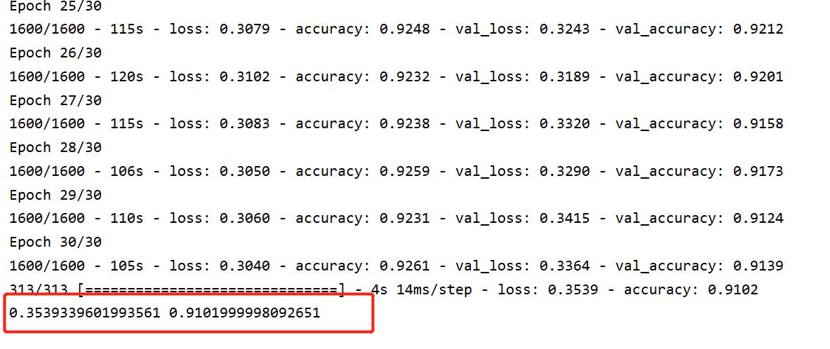
从训练日志中，可以看到 loss 一直在减小：

等待训练结束后看下评估模型的结果：

下面看下 tensorboard 中可视化的损失及准确率：

tensorboard --logdir=log/train

使用浏览器访问：http://localhost:6006/ 查看结果：

三、模型预测

上面搭建的模型，训练后会在 model 下生成 model.h5 模型，下面直接加载该模型进行预测：

import tensorflow as tf
import matplotlib.pyplot as plt

keras = tf.keras
fashion_mnist  = tf.keras.datasets.fashion_mnist
plt.rcParams['font.sans-serif'] = ['SimHei']

# 加载 MNIST 数据集
(x_train, y_train), (x_test, y_test) = fashion_mnist.load_data()
# 数据归一化
x_train, x_test = x_train / 255.0, x_test / 255.0

classify = 
    0: 'T恤/上衣',
    1: '裤子',
    2: '套头衫',
    3: '连衣裙',
    4: '外套',
    5: '凉鞋',
    6: '衬衫',
    7: '运动鞋',
    8: '包',
    9: '短靴'


model = keras.models.load_model('./model/model.h5')

for i in range(10):
    image = x_test[i]
    label = y_test[i]
    softmax = model.predict(image.reshape([1, 28, 28, 1]))
    y_label = tf.argmax(softmax, axis=1).numpy()[0]
    plt.imshow(image, cmap=plt.cm.gray)
    plt.title(label = ('预测结果: '+ classify[y_label] + ',  真实结果: '+ classify[label]))
    plt.show()