MobileNet V2 图像分类
Posted Henry_zhangs
tags:
篇首语:本文由小常识网(cha138.com)小编为大家整理,主要介绍了MobileNet V2 图像分类相关的知识,希望对你有一定的参考价值。
目录
2.1 Inverted Residuals 模块 + 线性激活
1. MobileNet V1 的不足
residual 残差模块的使用对网络的梯度更新很有帮助,可以加速网络的训练,以至于residual模块几乎成为了深度网络的标配。
因此,基于残差模块的优点,MobileNet V1 的第一个缺点就是没有引入residual block
其次很重要的是,经过实验证明,大部分训练出来的MobileNet V1里面的depthwise模块权重为零。这样不仅仅浪费了部分的资源,并且MobileNet V1本身参数量就很少, 权重为大部分为零对网络本身的性能也有影响。
并且,ReLU函数小于零的抑制性也会减少网络的参数
关于这部分的相关解释,因为depthwise深度卷积是单个2维的卷积核对单个channel进行卷积,所以可能忽略了空间尺度(channel)的信息。因为正常的卷积是3维的,这样包括了channel的信息,这样就类似于线性网络分类图像忽略了像素点的空间信息一样
2. MobileNet V2
MobileNet V2 介绍
2.1 Inverted Residuals 模块 + 线性激活
首先 MobileNet V2 解决了第一个问题,加入了残差结构,但是这里使用的是Inverted Residuals
如图,正常的残差块为了减少模型的参数量,用了1*1进行降维,最后为了shortcut可以拼接,再使用1*1进行升维。
而Inverted Residuals是利用1*1模块进行升维,最后在使用1*1进行降维实现shortcut的相加。因此这里的shortcut是连接在低维的bottleneck上
而另一个不同点是,正常残差块shortcut连接后,使用非线性函数ReLU进行激活。
因为Inverted Residuals本身维度就很小,本质上已经包含了非常重要的信息(manifold of interest),所以经过非线性激活(ReLU)会丢失信息,所以这里使用的是线性激活,y=x,也就是不加任何的激活函数
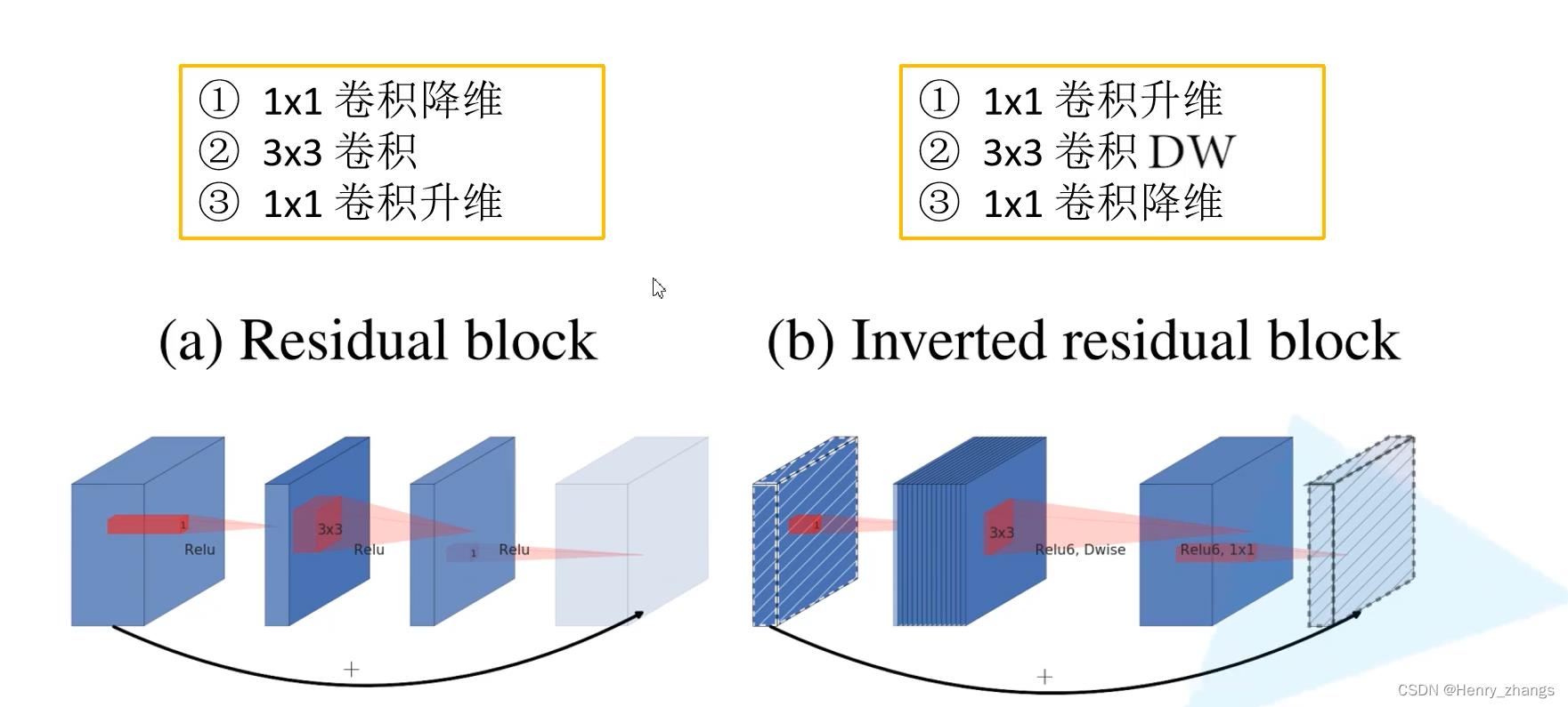
Inverted Residuals的连接如下:左边是深度可分离卷积,右边是Inverted Residuals(加了升维)
2.2 关于 Inverted Residuals 的解释
为什么需要1*1卷积进行升维呢?
论文中是这样解释的
首先,随着网络的深入,每层卷积的输出特征图(channel)会越来越多,而高维的特征图包含了主要的特征信息(论文中用manifold of interest表示)。然而,高维的信息是可以通过低维进行表示的,也就是说将高维度降维后,低维仍然可以表征所有的特征信息(manifold of interest)。
例如输出1024个特征图去表征提取到的信息,然而有一半的信息是冗余的,所以就可以用512去降维,达到减少参数的目的
MobileNet V1中的超参数α 就是控制输出channel的个数
超参数宽度乘数α:允许人们降低空间的维数(MobileNet V1的α就是控制channel的),直到感兴趣的流形跨越整个空间。
降维过度+relu(小于0,不输出,信息丢失)就会造成信息丢失,
如果要保证relu不丢失信息,输入应该全为正,但是这样relu就是一个线性的激活函数,失去了非线性能力。所以解决办法是,扩充出冗余的维度(inverted),在高维里面用relu。这样扩充多余的维度,ReLU就能保留manifold的信息
因此,低维度保留主要的manifold信息,升高维度用来做非线性变换,增加网络的非线性能力,所以 Inverted Residuals 的shortcut 要连接在低维。同时,为了保留低维的manifold信息,做线性变换就行了
低维度:bottleneck 包含主要信息,manifold of interest 扩充的高维:非线性变换能力,相当于将两者分离了
还有一种哲学思想的解释,低维的信息就相当于一个压缩文件,保留的特征的全部信息。扩充到高维(1*1升维)就是解压,然后对里面的信息进行处理(depthwise 深度卷积,非线性激活),最后再压缩(1*1降维)。所以主要的信息都在低维里,所以shortcut连接在低维
2.3 升维
如图:input 代表输入的信息,经过Inverted Residuals 模块
如果升高的维度是2的话,还原回原来的信息会丢失大部分的信息,当提升的维度逐渐变多时,信息就可以逐渐的还原

3. MobileNet V2 网络搭建
网络的模块如图

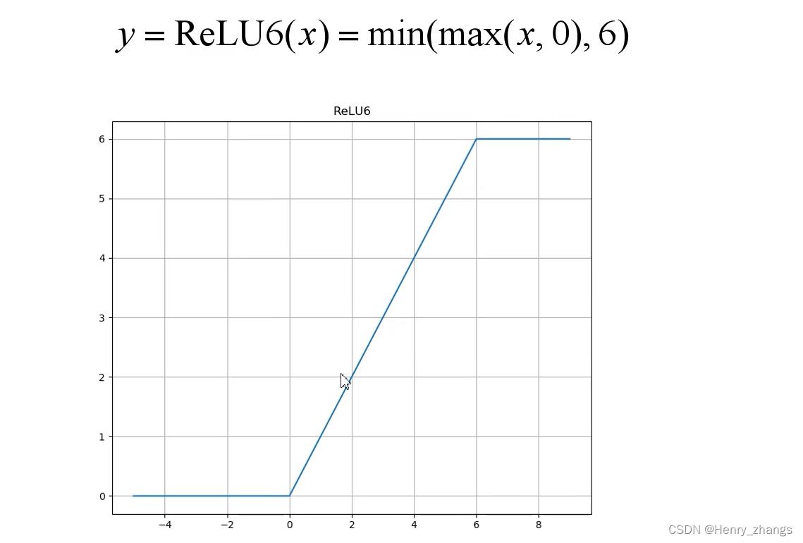
使用的非线性激活函数维ReLU6
其中bottleneck的设计方式为:

MobileNet V2 代码:
from torch import nn
import torch


# 保证用了α后,channel能被8整除
def _make_divisible(ch, divisor=8, min_ch=None):

    if min_ch is None:
        min_ch = divisor
    new_ch = max(min_ch, int(ch + divisor / 2) // divisor * divisor)
    # Make sure that round down does not go down by more than 10%.
    if new_ch < 0.9 * ch:
        new_ch += divisor
    return new_ch


# conv + BN + ReLU6
class ConvBNReLU(nn.Sequential):
    def __init__(self, in_channel, out_channel, kernel_size=3, stride=1, groups=1): # groups = 1代表普通卷积
        padding = (kernel_size - 1) // 2    # padding 设定为 same 卷积,通过stride将size减半
        super(ConvBNReLU, self).__init__(
            nn.Conv2d(in_channel, out_channel, kernel_size, stride, padding, groups=groups, bias=False),
            nn.BatchNorm2d(out_channel),
            nn.ReLU6(inplace=True)
        )


# 定义 invert residual
class InvertedResidual(nn.Module):
    def __init__(self, in_channel, out_channel, stride, expand_ratio):
        super(InvertedResidual, self).__init__()
        hidden_channel = in_channel * expand_ratio      # 升维的扩展因子
        self.use_shortcut = stride == 1 and in_channel == out_channel

        layers = []
        if expand_ratio != 1:
            # 1x1 pointwise conv
            layers.append(ConvBNReLU(in_channel, hidden_channel, kernel_size=1))
        layers.extend([
            # 3x3 depthwise conv        # groups = in_channel 就是 dw卷积
            ConvBNReLU(hidden_channel, hidden_channel, stride=stride, groups=hidden_channel),
            # 1x1 pointwise conv(linear)-----> y = x 不需要激活函数
            nn.Conv2d(hidden_channel, out_channel, kernel_size=1, bias=False),
            nn.BatchNorm2d(out_channel),
        ])

        self.conv = nn.Sequential(*layers)

    def forward(self, x):
        if self.use_shortcut:
            return x + self.conv(x)
        else:
            return self.conv(x)


# MobileNet V2 网络
class MobileNetV2(nn.Module):
    def __init__(self, num_classes=1000, alpha=1.0, round_nearest=8):
        super(MobileNetV2, self).__init__()
        block = InvertedResidual
        input_channel = _make_divisible(32 * alpha, round_nearest)
        last_channel = _make_divisible(1280 * alpha, round_nearest)

        inverted_residual_setting = [
            # t, c, n, s
            # t : 升维的倍数    c : 卷积核个数  n : 重复次数 s : 首个模块的步长
            [1, 16, 1, 1],
            [6, 24, 2, 2],
            [6, 32, 3, 2],
            [6, 64, 4, 2],
            [6, 96, 3, 1],
            [6, 160, 3, 2],
            [6, 320, 1, 1],
        ]

        features = []
        # conv1 layer
        features.append(ConvBNReLU(3, input_channel, stride=2))
        # building inverted residual residual blockes
        for t, c, n, s in inverted_residual_setting:
            output_channel = _make_divisible(c * alpha, round_nearest)
            for i in range(n):
                stride = s if i == 0 else 1
                features.append(block(input_channel, output_channel, stride, expand_ratio=t))
                input_channel = output_channel
        # building last several layers
        features.append(ConvBNReLU(input_channel, last_channel, 1))
        # combine feature layers
        self.features = nn.Sequential(*features)

        # building classifier
        self.avgpool = nn.AdaptiveAvgPool2d((1, 1))
        self.classifier = nn.Sequential(
            nn.Dropout(0.2),
            nn.Linear(last_channel, num_classes)
        )

        # weight initialization
        for m in self.modules():
            if isinstance(m, nn.Conv2d):
                nn.init.kaiming_normal_(m.weight, mode='fan_out')
                if m.bias is not None:
                    nn.init.zeros_(m.bias)
            elif isinstance(m, nn.BatchNorm2d):
                nn.init.ones_(m.weight)
                nn.init.zeros_(m.bias)
            elif isinstance(m, nn.Linear):
                nn.init.normal_(m.weight, 0, 0.01)
                nn.init.zeros_(m.bias)

    def forward(self, x):
        x = self.features(x)
        x = self.avgpool(x)
        x = torch.flatten(x, 1)
        x = self.classifier(x)
        return x
网络的结构可以通过torchsummary观察:

4. 迁移学习分类CIFAR10 数据集
预训练权重在这里查看,可以通过 url 搜索

代码:
import json
import torch
import torch.nn as nn
import torch.optim as optim
from torchvision import transforms, datasets
from tqdm import tqdm
from model import MobileNetV2
from torch.utils.data import DataLoader
# 超参数
DEVICE = torch.device("cuda:0" if torch.cuda.is_available() else "cpu")
BATCH_SIZE = 16
EPOCHS = 2
PRE_MODEL_WEIGHT = './mobilenet_v2-b0353104.pth'
SAVE_PATH_WIGHT = './MobileNetV2.pth'
LEARNING_RATE = 0.001
# 预处理
data_transform =
"train": transforms.Compose([transforms.RandomResizedCrop(224),
transforms.RandomHorizontalFlip(),
transforms.ToTensor(),
transforms.Normalize([0.485, 0.456, 0.406], [0.229, 0.224, 0.225])]),
"test": transforms.Compose([transforms.Resize(256),
transforms.CenterCrop(224),
transforms.ToTensor(),
transforms.Normalize([0.485, 0.456, 0.406], [0.229, 0.224, 0.225])])
# 载入训练集
train_dataset = datasets.CIFAR10(root='./data', train=True,transform=data_transform['train']) # 下载数据集
train_loader = DataLoader(train_dataset, batch_size=BATCH_SIZE, shuffle=True) # 读取数据集
# 载入测试集
test_dataset = datasets.CIFAR10(root='./data', train=False,transform=data_transform['test']) # 下载数据集
test_loader = DataLoader(test_dataset, batch_size=BATCH_SIZE, shuffle=False) # 读取数据集
# 样本个数
num_train = len(train_dataset) # 50000
num_test = len(test_dataset) # 10000
# 类别和 label
dataSetClasses = train_dataset.class_to_idx
# 'airplane': 0, 'automobile': 1, 'bird': 2, 'cat': 3, 'deer': 4, 'dog': 5, 'frog': 6, 'horse': 7, 'ship': 8, 'truck': 9
class_dict = dict((val, key) for key, val in dataSetClasses.items())
# 0: 'airplane', 1: 'automobile', 2: 'bird', 3: 'cat', 4: 'deer', 5: 'dog', 6: 'frog', 7: 'horse', 8: 'ship', 9: 'truck'
json_str = json.dumps(class_dict, indent=4)
'''
"0": "airplane",
"1": "automobile",
"2": "bird",
"3": "cat",
"4": "deer",
"5": "dog",
"6": "frog",
"7": "horse",
"8": "ship",
"9": "truck"
'''
with open('class_indices.json', 'w') as json_file:
json_file.write(json_str)
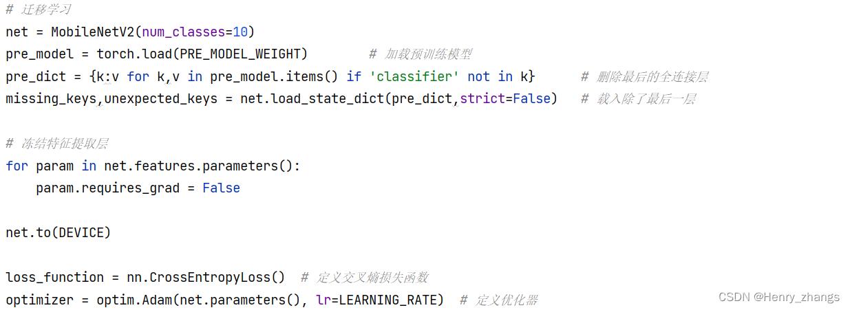
# 迁移学习
net = MobileNetV2(num_classes=10)
pre_model = torch.load(PRE_MODEL_WEIGHT) # 加载预训练模型
pre_dict = k:v for k,v in pre_model.items() if 'classifier' not in k # 删除最后的全连接层
missing_keys,unexpected_keys = net.load_state_dict(pre_dict,strict=False) # 载入除了最后一层
# 冻结特征提取层
for param in net.features.parameters():
param.requires_grad = False
net.to(DEVICE)
loss_function = nn.CrossEntropyLoss() # 定义交叉熵损失函数
optimizer = optim.Adam(net.parameters(), lr=LEARNING_RATE) # 定义优化器
# train
best_acc = 0.0
for epoch in range(EPOCHS):
net.train() # 开启dropout
running_loss = 0.0
for images, labels in tqdm(train_loader):
images, labels = images.to(DEVICE), labels.to(DEVICE)
optimizer.zero_grad() # 梯度下降
outputs = net(images) # 前向传播
loss = loss_function(outputs, labels) # 计算损失
loss.backward() # 反向传播
optimizer.step() # 梯度更新
running_loss += loss.item()
# test
net.eval() # 关闭dropout
acc = 0.0
with torch.no_grad():
for x, y in tqdm(test_loader):
x, y = x.to(DEVICE), y.to(DEVICE)
outputs = net(x)
predicted = torch.max(outputs, dim=1)[1]
acc += (predicted == y).sum().item()
accurate = acc / num_test # 计算正确率
train_loss = running_loss / num_train # 计算损失
print('[epoch %d] train_loss: %.3f test_accuracy: %.3f' %
(epoch + 1, train_loss, accurate))
if accurate > best_acc:
best_acc = accurate
torch.save(net.state_dict(), SAVE_PATH_WIGHT)
print('Finished Training....')
这里需要注意的是,实例化网络的时候,已经将网络的结构改变了(num_classes=10),所以预训练权重是对应不上的,因此这里要将最后一个全连接层去掉,然后不完全匹配进行迁移读取参数
然后将特征提取层进行冻结,只训练后面的全连接层即可
这里的优化器没有进行更新,也可以实现
删出最后的全连接层,if 那块要看网络是如何定义的,因为原网络是self.classifier,如果定义的是self.fc 要么if 里面也要改变

5. 网络在CIFAR10 上的表现
代码:
import os
os.environ['KMP_DUPLICATE_LIB_OK'] = 'True'

import torch
import numpy as np
import matplotlib.pyplot as plt
from model import MobileNetV2
from torchvision.transforms import transforms
from torch.utils.data import DataLoader
import torchvision

classes = ('plane', 'car', 'bird', 'cat', 'deer', 'dog', 'frog', 'horse', 'ship', 'truck')

# 预处理
transformer = transforms.Compose([transforms.Resize(256),  # 保证比例不变,短边变为256
                                  transforms.CenterCrop(224),
                                  transforms.ToTensor(),
                                  transforms.Normalize([0.485, 0.456, 0.406], [0.229, 0.224, 0.255])])

# 加载模型
DEVICE = 'cuda' if torch.cuda.is_available() else 'cpu'
model = MobileNetV2(num_classes=10)
model.load_state_dict(torch.load('./MobileNetV2.pth'))
model.to(DEVICE)

# 加载数据
testSet = torchvision.datasets.CIFAR10(root='./data', train=False, download=False, transform=transformer)
testLoader = DataLoader(testSet, batch_size=12, shuffle=True)

# 获取一批数据
imgs, labels = next(iter(testLoader))
imgs = imgs.to(DEVICE)

# show
with torch.no_grad():
    model.eval()
    prediction = model(imgs)  # 预测
    prediction = torch.max(prediction, dim=1)[1]
    prediction = prediction.data.cpu().numpy()

    plt.figure(figsize=(12, 8))
    for i, (img, label) in enumerate(zip(imgs, labels)):
        x = np.transpose(img.data.cpu().numpy(), (1, 2, 0))  # 图像
        x[:, :, 0] = x[:, :, 0] * 0.229 + 0.485  # 去 normalization
        x[:, :, 1] = x[:, :, 1] * 0.224 + 0.456  # 去 normalization
        x[:, :, 2] = x[:, :, 2] * 0.255 + 0.406  # 去 normalization
        y = label.numpy().item()  # label
        plt.subplot(3, 4, i + 1)
        plt.axis(False)
        plt.imshow(x)
        plt.title('R:,P:'.format(classes[y], classes[prediction[i]]))
    plt.show()
结果展示:
Pytorch CIFAR10图像分类 MobileNet v1篇
Pytorch CIFAR10图像分类 MobileNet v1篇
文章目录
4.定义网络(MobileNet v1)
在之前的文章中讲的AlexNet、VGG、GoogLeNet以及ResNet网络,它们都是传统卷积神经网络(都是使用的传统卷积层),缺点在于内存需求大、运算量大导致无法在移动设备以及嵌入式设备上运行。而本文要讲的MobileNet网络就是专门为移动端,嵌入式端而设计。
我也看了论文,如果想仔细研究一下MobileNet的话,可以看我的另一篇博客【论文泛读】轻量化之MobileNets: Efficient Convolutional Neural Networks for Mobile Vision Applications
MobileNet网络是由google团队在2017年提出的,专注于移动端或者嵌入式设备中的轻量级CNN网络。相比传统卷积神经网络,在准确率小幅降低的前提下大大减少模型参数与运算量。(相比VGG16准确率减少了0.9%,但模型参数只有VGG的1/32)。
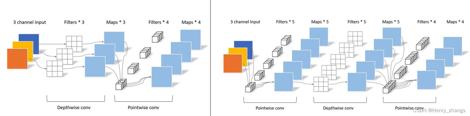
要说MobileNet网络的优点,无疑是其中的Depthwise Convolution结构(大大减少运算量和参数数量)。下图展示了传统卷积与DW卷积的差异,在传统卷积中,每个卷积核的channel与输入特征矩阵的channel相等(每个卷积核都会与输入特征矩阵的每一个维度进行卷积运算)。而在DW卷积中,每个卷积核的channel都是等于1的(每个卷积核只负责输入特征矩阵的一个channel,故卷积核的个数必须等于输入特征矩阵的channel数,从而使得输出特征矩阵的channel数也等于输入特征矩阵的channel数)
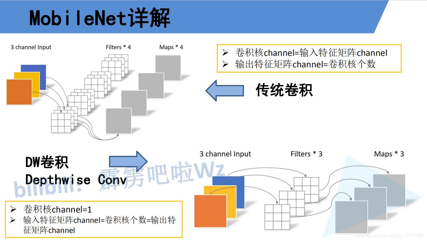
刚刚说了使用DW卷积后输出特征矩阵的channel是与输入特征矩阵的channel相等的,如果想改变/自定义输出特征矩阵的channel,那只需要在DW卷积后接上一个PW卷积即可,如下图所示,其实PW卷积就是普通的卷积而已(只不过卷积核大小为1)。通常DW卷积和PW卷积是放在一起使用的,一起叫做Depthwise Separable Convolution(深度可分卷积)。

那Depthwise Separable Convolution(深度可分卷积)与传统的卷积相比有到底能节省多少计算量呢,下图对比了这两个卷积方式的计算量,其中Df是输入特征矩阵的宽高(这里假设宽和高相等),Dk是卷积核的大小,M是输入特征矩阵的channel,N是输出特征矩阵的channel,卷积计算量近似等于卷积核的高 x 卷积核的宽 x 卷积核的channel x 输入特征矩阵的高 x 输入特征矩阵的宽(这里假设stride等于1),在我们mobilenet网络中DW卷积都是是使用3x3大小的卷积核。所以理论上普通卷积计算量是DW+PW卷积的8到9倍(公式来源于原论文):

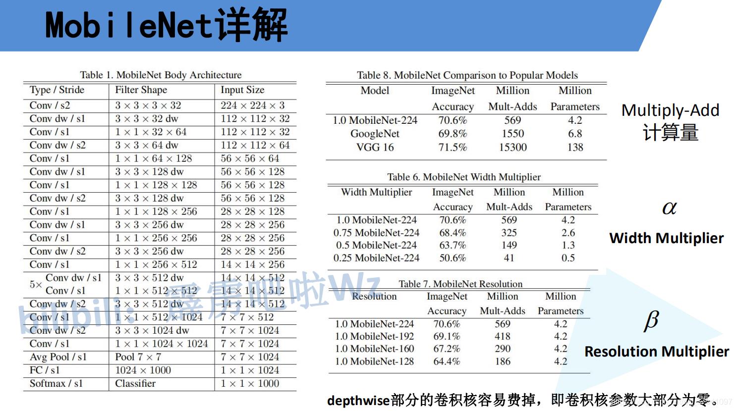
在了解完Depthwise Separable Convolution(深度可分卷积)后在看下mobilenet v1的网络结构,左侧的表格是mobileNetv1的网络结构,表中标Conv的表示普通卷积,Conv dw代表刚刚说的DW卷积,s表示步距,根据表格信息就能很容易的搭建出mobileNet v1网络。在mobilenetv1原论文中,还提出了两个超参数,一个是α一个是β。α参数是一个倍率因子,用来调整卷积核的个数,β是控制输入网络的图像尺寸参数,下图右侧给出了使用不同α和β网络的分类准确率,计算量以及模型参数:

首先我们还是得判断是否可以利用GPU,因为GPU的速度可能会比我们用CPU的速度快20-50倍左右,特别是对卷积神经网络来说,更是提升特别明显。
device = 'cuda' if torch.cuda.is_available() else 'cpu'
接着我们可以定义网络,在pytorch之中,定义我们的深度可分离卷积来说,我们需要调一个groups参数,就可以构建深度可分离卷积了。
class Block(nn.Module):
    '''Depthwise conv + Pointwise conv'''
    def __init__(self,in_channels,out_channels,stride=1):
        super(Block,self).__init__()
        # groups参数就是深度可分离卷积的关键
        self.conv1 = nn.Conv2d(in_channels,in_channels,kernel_size=3,stride=stride,
                               padding=1,groups=in_channels,bias=False)
        self.bn1 = nn.BatchNorm2d(in_channels)
        self.relu1 = nn.ReLU()
        self.conv2 = nn.Conv2d(in_channels,out_channels,kernel_size=1,stride=1,padding=0,bias=False)
        self.bn2 = nn.BatchNorm2d(out_channels)
        self.relu2 = nn.ReLU()
    def forward(self,x):
        x = self.relu1(self.bn1(self.conv1(x)))
        x = self.relu2(self.bn2(self.conv2(x)))
        return x

# 深度可分离卷积 DepthWise Separable Convolution
class MobileNetV1(nn.Module):
    # (128,2) means conv channel=128, conv stride=2, by default conv stride=1
    cfg = [64,(128,2),128,(256,2),256,(512,2),512,512,512,512,512,(1024,2),1024]

    def __init__(self, num_classes=10,alpha=1.0,beta=1.0):
        super(MobileNetV1,self).__init__()
        self.conv1 = nn.Sequential(
            nn.Conv2d(3,32,kernel_size=3,stride=1,bias=False),
            nn.BatchNorm2d(32),
            nn.ReLU()
        )
        self.avg = nn.AvgPool2d(kernel_size=2)
        self.layers = self._make_layers(in_channels=32)
        self.linear = nn.Linear(1024,num_classes)

    def _make_layers(self, in_channels):
        layers = []
        for x in self.cfg:
            out_channels = x if isinstance(x,int) else x[0]
            stride = 1 if isinstance(x,int) else x[1]
            layers.append(Block(in_channels,out_channels,stride))
            in_channels = out_channels
        return nn.Sequential(*layers)

    def forward(self,x):
        x = self.conv1(x)
        x = self.layers(x)
        x = self.avg(x)
        x = x.view(x.size()[0],-1)
        x = self.linear(x)
        return x
net = MobileNetV1(num_classes=10).to(device)
summary(net,(2,3,32,32))
========================================================================================== Layer (type:depth-idx) Output Shape Param # ========================================================================================== MobileNetV1 -- -- ├─Sequential: 1-1 [2, 32, 30, 30] -- │ └─Conv2d: 2-1 [2, 32, 30, 30] 864 │ └─BatchNorm2d: 2-2 [2, 32, 30, 30] 64 │ └─ReLU: 2-3 [2, 32, 30, 30] -- ├─Sequential: 1-2 [2, 1024, 2, 2] -- │ └─Block: 2-4 [2, 64, 30, 30] -- │ │ └─Conv2d: 3-1 [2, 32, 30, 30] 288 │ │ └─BatchNorm2d: 3-2 [2, 32, 30, 30] 64 │ │ └─ReLU: 3-3 [2, 32, 30, 30] -- │ │ └─Conv2d: 3-4 [2, 64, 30, 30] 2,048 │ │ └─BatchNorm2d: 3-5 [2, 64, 30, 30] 128 │ │ └─ReLU: 3-6 [2, 64, 30, 30] -- │ └─Block: 2-5 [2, 128, 15, 15] -- │ │ └─Conv2d: 3-7 [2, 64, 15, 15] 576 │ │ └─BatchNorm2d: 3-8 [2, 64, 15, 15] 128 │ │ └─ReLU: 3-9 [2, 64, 15, 15] -- │ │ └─Conv2d: 3-10 [2, 128, 15, 15] 8,192 │ │ └─BatchNorm2d: 3-11 [2, 128, 15, 15] 256 │ │ └─ReLU: 3-12 [2, 128, 15, 15] -- │ └─Block: 2-6 [2, 128, 15, 15] -- │ │ └─Conv2d: 3-13 [2, 128, 15, 15] 1,152 │ │ └─BatchNorm2d: 3-14 [2, 128, 15, 15] 256 │ │ └─ReLU: 3-15 [2, 128, 15, 15] -- │ │ └─Conv2d: 3-16 [2, 128, 15, 15] 16,384 │ │ └─BatchNorm2d: 3-17 [2, 128, 15, 15] 256 │ │ └─ReLU: 3-18 [2, 128, 15, 15] -- │ └─Block: 2-7 [2, 256, 8, 8] -- │ │ └─Conv2d: 3-19 [2, 128, 8, 8] 1,152 │ │ └─BatchNorm2d: 3-20 [2, 128, 8, 8] 256 │ │ └─ReLU: 3-21 [2, 128, 8, 8] -- │ │ └─Conv2d: 3-22 [2, 256, 8, 8] 32,768 │ │ └─BatchNorm2d: 3-23 [2, 256, 8, 8] 512 │ │ └─ReLU: 3-24 [2, 256, 8, 8] -- │ └─Block: 2-8 [2, 256, 8, 8] -- │ │ └─Conv2d: 3-25 [2, 256, 8, 8] 2,304 │ │ └─BatchNorm2d: 3-26 [2, 256, 8, 8] 512 │ │ └─ReLU: 3-27 [2, 256, 8, 8] -- │ │ └─Conv2d: 3-28 [2, 256, 8, 8] 65,536 │ │ └─BatchNorm2d: 3-29 [2, 256, 8, 8] 512 │ │ └─ReLU: 3-30 [2, 256, 8, 8] -- │ └─Block: 2-9 [2, 512, 4, 4] -- │ │ └─Conv2d: 3-31 [2, 256, 4, 4] 2,304 │ │ └─BatchNorm2d: 3-32 [2, 256, 4, 4] 512 │ │ └─ReLU: 3-33 [2, 256, 4, 4] -- │ │ └─Conv2d: 3-34 [2, 512, 4, 4] 131,072 │ │ └─BatchNorm2d: 3-35 [2, 512, 4, 4] 1,024 │ │ └─ReLU: 3-36 [2, 512, 4, 4] -- │ └─Block: 2-10 [2, 512, 4, 4] -- │ │ └─Conv2d: 3-37 [2, 512, 4, 4] 4,608 │ │ └─BatchNorm2d: 3-38 [2, 512, 4, 4] 1,024 │ │ └─ReLU: 3-39 [2, 512, 4, 4] -- │ │ └─Conv2d: 3-40 [2, 512, 4, 4] 262,144 │ │ └─BatchNorm2d: 3-41 [2, 512, 4, 4] 1,024 │ │ └─ReLU: 3-42 [2, 512, 4, 4] -- │ └─Block: 2-11 [2, 512, 4, 4] -- │ │ └─Conv2d: 3-43 [2, 512, 4, 4] 4,608 │ │ └─BatchNorm2d: 3-44 [2, 512, 4, 4] 1,024 │ │ └─ReLU: 3-45 [2, 512, 4, 4] -- │ │ └─Conv2d: 3-46 [2, 512, 4, 4] 262,144 │ │ └─BatchNorm2d: 3-47 [2, 512, 4, 4] 1,024 │ │ └─ReLU: 3-48 [2, 512, 4, 4] -- │ └─Block: 2-12 [2, 512, 4, 4] -- │ │ └─Conv2d: 3-49 [2, 512, 4, 4]