CS224W(task12)GAT & GNN training tips

Posted 2023-04-02 山顶夕景

note

• GAT使用attention对线性转换后的节点进行加权求和：利用自身节点的特征向量分别和邻居节点的特征向量，进行内积计算score。
• 异质图的消息传递和聚合：$${\mathbf{h}}_v^{(l+1)}=\sigma \left(\sum _{r\in R}\sum _{u\in N_v^r}\frac{1}{c_{v,r}}{\mathbf{W}}_r^{(l)}{\mathbf{h}}_u^{(l)}+{\mathbf{W}}_0^{(l)}{\mathbf{h}}_v^{(l)}\right)$$

文章目录

• note
• 一、GAT model
• 二、GNN模型训练要点
• • 1. Graph Manipulation
  • 2. GNN training
  • • （1）Node-level
    • （2）Edge-level
    • （3）Graph-level
  • 3. Issue of Global pooling
  • • （1）Global pooling的毛病
    • （2）DidffPool 社群分层池化：
• 三、GNN training tips
• • 3.1 Spliting Graphs is special
  • 3.2 异质图 Heterogeneous graph
• 附：时间安排
• Reference

一、GAT model

图注意神经网络（GAT）来源于论文 Graph Attention Networks。其数学定义为，
$${\mathbf{x}}_i^{\prime }={\alpha }_{i,i}\mathbf{\Theta }{\mathbf{x}}_i+\sum _{j\in \mathcal{N}(i)}{\alpha }_{i,j}\mathbf{\Theta }{\mathbf{x}}_j,$$
GAT和所有的attention mechanism一样，GAT的计算也分为两步走：
（1）计算注意力系数（attention coefficient）：（下图来自《GRAPH ATTENTION NETWORKS》）
其中注意力系数${\alpha }_{i,j}$的计算方法为，
$${\alpha }_{i,j}=\frac{\exp \left(\mathrm{LeakyReLU}\left({\mathbf{a}}^{\top }[\mathbf{\Theta }{\mathbf{x}}_i\Vert \mathbf{\Theta }{\mathbf{x}}_j]\right)\right)}{{\sum }_{k\in \mathcal{N}(i)\cup i}\exp \left(\mathrm{LeakyReLU}\left({\mathbf{a}}^{\top }[\mathbf{\Theta }{\mathbf{x}}_i\Vert \mathbf{\Theta }{\mathbf{x}}_k]\right)\right)}.$$

（2）加权求和（aggregate）：根据（1）的系数，把特征加权求和（aggregate）$${\mathbf{h}}_v^{(l)}=\sigma \left(\sum _{u\in N(v)}{\alpha }_{vu}{\mathbf{W}}^{(l)}{\mathbf{h}}_u^{(l-1)}\right)$$

二、GNN模型训练要点

1. Graph Manipulation

• feature manipulation：feature augmentation, such as we can use cycle count as augmented node features
• struture manipulation：
  • sparse graph: add virtual nodes or edges
  • dense graph: sample neighbors when doing message passing
  • large graph: sample subgraphs to compute embeddings

2. GNN training

（1）Node-level

• After GNN computation, we have $d$-dim node
  $$\text{ embeddings: }{\mathbf{h}}_v^{(L)}\in {\mathbb{R}}^d,\forall v\in G$$
• such as k-way prediction：
• ${\hat{\mathbf{y}}}_v={\mathrm{Head}}_{\text{node }}\left({\mathbf{h}}_v^{(L)}\right)={\mathbf{W}}^{(H)}{\mathbf{h}}_v^{(L)}$
  • ${\mathbf{W}}^{(H)}\in {\mathbb{R}}^{k\ast d}$ : We map node embeddings from ${\mathbf{h}}_v^{(L)}\in {\mathbb{R}}^d$ to ${\hat{y}}_v\in {\mathbb{R}}^k$
  • compute the loss

（2）Edge-level

• use pairs of node embeddings
• such as k-way prediction： y ^ u v = Head

  图注意网络GAT理解及Pytorch代码实现PyGAT代码详细注释

  文章目录

  • • GAT
    • 代码实现【PyGAT】
    • • GraphAttentionLayer【一个图注意力层实现】
      • 用上面实现的单层网络测试
      • 加入Multi-head机制的GAT
      • 对数据集Cora的处理
      • csr_matrix()处理稀疏矩阵
      • encode_onehot()对label编号
      • build graph
      • 邻接矩阵构造
    • GAT的推广

  GAT

  题：Graph Attention Networks
  摘要：
  提出了图形注意网络(GAT) ，这是一种基于图结构数据的新型神经网络结构，利用掩蔽的自我注意层来解决基于图卷积或其近似的先前方法的缺点。通过叠加层，节点能够参与其邻域的特征，我们能够(隐式地)为邻域中的不同节点指定不同的权重，而不需要任何代价高昂的矩阵操作(如反演) ，或者依赖于预先知道图的结构。通过这种方法，我们同时解决了基于谱的图形神经网络的几个关键问题，并使我们的模型容易地适用于归纳和转导问题。我们的 GAT 模型已经实现或匹配了四个已建立的转导和归纳图基准的最新结果: Cora，Citeseer 和 Pubmed 引用网络数据集，以及protein-protein interaction dataset(其中测试图在训练期间保持不可见)。

  在Paper with code 网址，可找到对应论文和github源码，原论文使用TensorFlow实现，本篇主要对Pytorch版本的 PyGAT附详细注释帮助理解和测试。

  GitHUb: keras版本实现
  Pytorch版本实现 PyGAT

  
  

  截图及下文代码注释参考自视频：GAT详解及代码实现

  视频中的eij的实现与源码不同，视频中是先拼接两个W，再与a乘；
  源码在_prepare_attentional_mechanism_input()函数中先分别与a乘，再拼接。

  代码实现【PyGAT】

  在PyGAT ：

  • layers.py中定义Simple GAT layer实现（GraphAttentionLayer）和Sparse version GAT layer实现（SpGraphAttentionLayer）。
  • models.py 实现两个版本加入Multi-head机制
  • trains.py 使用model定义的GAT构建模型进行训练，使用cora数据集

  GraphAttentionLayer【一个图注意力层实现】

  class GraphAttentionLayer(nn.Module):
      """
      Simple GAT layer, similar to https://arxiv.org/abs/1710.10903
      """
      def __init__(self, in_features, out_features, dropout, alpha, concat=True):
          super(GraphAttentionLayer, self).__init__()
          self.dropout = dropout
          self.in_features = in_features#结点向量的特征维度
          self.out_features = out_features#经过GAT之后的特征维度
          self.alpha = alpha#dropout参数
          self.concat = concat#LeakyReLU参数
  
          # 定义可训练参数，即论文中的W和a
          self.W = nn.Parameter(torch.empty(size=(in_features, out_features)))
          nn.init.xavier_uniform_(self.W.data, gain=1.414)# xavier初始化
          self.a = nn.Parameter(torch.empty(size=(2*out_features, 1)))
          nn.init.xavier_uniform_(self.a.data, gain=1.414)# xavier初始化
  
          # 定义leakyReLU激活函数
          self.leakyrelu = nn.LeakyReLU(self.alpha)
  
      def forward(self, h, adj):
          '''
          adj图邻接矩阵，维度[N,N]非零即一
          h.shape: (N, in_features), self.W.shape:(in_features,out_features)
          Wh.shape: (N, out_features)
          '''
          Wh = torch.mm(h, self.W) # 对应eij的计算公式
          e = self._prepare_attentional_mechanism_input(Wh)#对应LeakyReLU(eij)计算公式
  
          zero_vec = -9e15*torch.ones_like(e)#将没有链接的边设置为负无穷
          attention = torch.where(adj > 0, e, zero_vec)#[N,N]
          # 表示如果邻接矩阵元素大于0时，则两个节点有连接，该位置的注意力系数保留
          # 否则需要mask设置为非常小的值，因为softmax的时候这个最小值会不考虑
          attention = F.softmax(attention, dim=1)# softmax形状保持不变[N,N]，得到归一化的注意力全忠！
          attention = F.dropout(attention, self.dropout, training=self.training)# dropout,防止过拟合
          h_prime = torch.matmul(attention, Wh)#[N,N].[N,out_features]=>[N,out_features]
  
          # 得到由周围节点通过注意力权重进行更新后的表示
          if self.concat:
              return F.elu(h_prime)
          else:
              return h_prime
  
      def _prepare_attentional_mechanism_input(self, Wh):
          # Wh.shape (N, out_feature)
          # self.a.shape (2 * out_feature, 1)
          # Wh1&2.shape (N, 1)
          # e.shape (N, N)
          # 先分别与a相乘再进行拼接
          Wh1 = torch.matmul(Wh, self.a[:self.out_features, :])
          Wh2 = torch.matmul(Wh, self.a[self.out_features:, :])
          # broadcast add
          e = Wh1 + Wh2.T
          return self.leakyrelu(e)
  
      def __repr__(self):
          return self.__class__.__name__ + ' (' + str(self.in_features) + ' -> ' + str(self.out_features) + ')'
  
  

  用上面实现的单层网络测试

  x = torch.randn(6,10)
  adj=torch.tensor([[0,1,1,0,0,0],
                    [1,0,1,0,0,0],
                    [1,1,0,1,0,0],
                    [0,0,1,0,1,1],
                    [0,0,0,1,0,0,],
                    [0,0,0,1,1,0]])
  my_gat = GraphAttentionLayer(10,5,0.2,0.2)
  print(my_gat(x,adj))
  

  输出：
  tensor([[-0.2965,  2.8110, -0.6680, -0.9643, -0.9882],
          [ 0.0000,  0.0000,  0.0000,  0.0000,  0.0000],
          [-0.4981, -0.7515,  1.1159,  0.3546,  1.3592],
          [ 0.4679,  1.7208,  0.3084, -0.5331, -0.1291],
          [-0.4375, -0.8778,  1.1767, -0.5869,  1.5154],
          [-0.2164, -0.5897,  0.4988, -0.3125,  0.6423]], grad_fn=<EluBackward>)
  

  加入Multi-head机制的GAT

  用不同head捕捉不同特征，使模型有更好的拟合能力。

  class GAT(nn.Module):
      def __init__(self, nfeat, nhid, nclass, dropout, alpha, nheads):
          """Dense version of GAT."""
          super(GAT, self).__init__()
          self.dropout = dropout
  
          # 加入Multi-head机制
          self.attentions = [GraphAttentionLayer(nfeat, nhid, dropout=dropout, alpha=alpha, concat=True) for _ in range(nheads)]
          for i, attention in enumerate(self.attentions):
              self.add_module('attention_'.format(i), attention)
  
          self.out_att = GraphAttentionLayer(nhid * nheads, nclass, dropout=dropout, alpha=alpha, concat=False)
  
      def forward(self, x, adj):
          x = F.dropout(x, self.dropout, training=self.training)
          x = torch.cat([att(x, adj) for att in self.attentions], dim=1)
          x = F.dropout(x, self.dropout, training=self.training)
          x = F.elu(self.out_att(x, adj))
          return F.log_softmax(x, dim=1)
  
  

  对数据集Cora的处理

  
  数据集中两个文件，cites：比如上图11行：编号25和编号1114331的文章
  content文件：如下图，每篇文章的id、features及类别
  

  csr_matrix()处理稀疏矩阵

  utils.py中对数据进行的处理

  #数据是稀疏的，csr_matrix操作从行开始将1的位置取出来,对数据进行压缩

  features = sp.csr_matrix(idx_features_labels[:, 1:-1], dtype=np.float32)
  labels = encode_onehot(idx_features_labels[:, -1])
  

  

  encode_onehot()对label编号

  有7个类别，通过classes_dict是7*7的对角阵把每个类别映射成不同向量，对所有label进行编号，再将编号转换为one_hot向量
  

  def encode_onehot(labels):
      # The classes must be sorted before encoding to enable static class encoding.
      # In other words, make sure the first class always maps to index 0.
      classes = sorted(list(set(labels)))
      classes_dict = c: np.identity(len(classes))[i, :] for i, c in enumerate(classes)
      labels_onehot = np.array(list(map(classes_dict.get, labels)), dtype=np.int32)
      return labels_onehot
  

  build graph

  见注释：

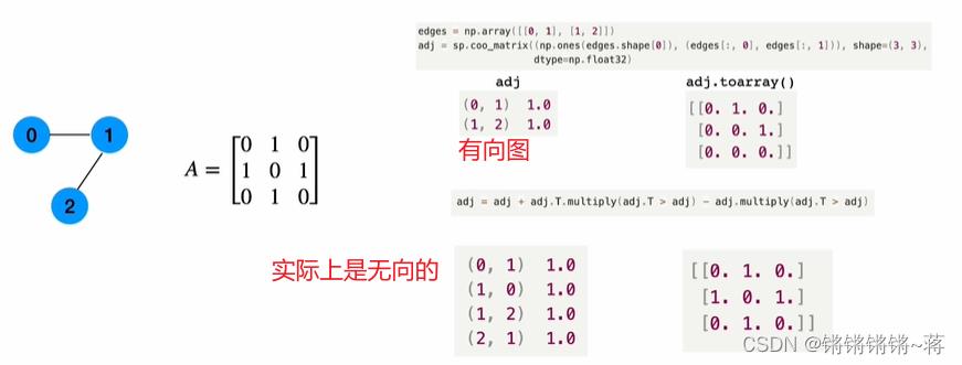
  # build graph
      idx = np.array(idx_features_labels[:, 0], dtype=np.int32)#获取所有文章id
      idx_map = j: i for i, j in enumerate(idx)#按文章数目，对id重新映射
      # 读取数据集中文章和文章直接的引用关系
      edges_unordered = np.genfromtxt(".cites".format(path, dataset), dtype=np.int32)
      # 根据idx_map,将文章引用关系也重新映射
      edges = np.array(list(map(idx_map.get, edges_unordered.flatten())), dtype=np.int32).reshape(edges_unordered.shape)
      adj = sp.coo_matrix((np.ones(edges.shape[0]), (edges[:, 0], edges[:, 1])), shape=(labels.shape[0], labels.shape[0]), dtype=np.float32)
  
      # build symmetric adjacency matrix 生成邻接矩阵
      adj = adj + adj.T.multiply(adj.T > adj) - adj.multiply(adj.T > adj)
  
      features = normalize_features(features)
      adj = normalize_adj(adj + sp.eye(adj.shape[0]))
  
  

  邻接矩阵构造

  csr_matrix()只记录了（0，1）1,忽略了（1，0）1。所以需要coo_matrix()操作！才能还原出无向图的邻接矩阵！
  

  本文的一些代码注释及截图还可见视频

  一个拓展：

  GAT的推广

  GAT的推广
  GAT仅仅是应用在了单层图结构网络上，我们是否可以将它推广到多层网络结构呢？

  这里我们假设一个有N层网络的结构，每层网络都定义了相同的节点，但是节点之间的关系有所差异。举一个简单的例子，假设有一个用户关系型网络，每层网络的节点都被定义成了网络中的用户，网络的第一层视图的关系可以定义为，两个用户之间是否具有好友关系；网络的第二层视图可以定义为，你评论过我的动态；网络的第三层视图可以定义为你转发过我的动态；第四层关系可以定义为，你at过我等等。

  通过这样的定义我们就完成了一个多层网络的构建，他们共享相同的节点，但又分别具有不同的邻边，如果我们分别处理每一层视图视图，然后将他们得出的节点表示单纯相加的话，就可能会失去不同视图之间的协作关系，降低分类（预测）的精度。

  基于以上观点，我们提出了一种新的方法：首先在每一层单视图中应用GAT进行学习，并计算出每层视图的节点表示。之后再不同视图之间引入attention机制来让网络自行学习不同视图的权重。之后根据学习的权重，将各个视图加权相加得到全局节点表示并进行后续的诸如节点表示，链接预测等任务。

  同时，因为不同视图共享同样的节点，即使每一层视图都表示了不同的节点关系，最终得到的每一层的节点嵌入表示应具有一定的相关性。基于以上理论，我们在每层GAT的网络参数间引入正则化项来约束参数，使其向互相相近的方向学习。大致的网络流程图如下：

  这部分来源于 链接：https://www.jianshu.com/p/d5d366ba1a57 来源：简书

  以上是关于CS224W(task12)GAT & GNN training tips的主要内容，如果未能解决你的问题，请参考以下文章

  CS224W摘要12.Frequent Subgraph Mining with GNNs

  CS224W摘要06.07.GNN

  学习笔记CS224W速记（图模型专题）

  学习笔记CS224W速记（图模型专题）

  学习笔记CS224W速记（图模型专题）

  学习笔记CS224W速记（图模型专题）