吴恩达_MIT_MachineLearning公开课ch01

Posted 2022-12-04 给个HK.phd读

之前一直和Tensorflow、PyTorch一些框架进行纠缠。现在显然幡然醒悟，这样是不对的，我们不是去学怎么搭别人的顺风车，我们要做的是自己造轮子造车。

任何课程评价都可以说是对这一门五星级课程的亵渎了。

概念

讲述了机器学习的几种模式，包括了监督学习、无监督学习、半监督学习等。
监督学习就是我们知道了输入与输出的关系，比如等会作业里要做的假设了一个代价函数，而我们的目标就是不断去缩小这个损失。
其他的先不说，这一章主要讲的就是监督学习下的回归问题，而且是线性回归，也就是Linear regression。

代价函数

代价函数其实就是我们的损失函数。
我们在框架内应该用过许多“XXXLoss”，吴老师这里着重讲了个BCELoss。
也就是我们的均值平方差？

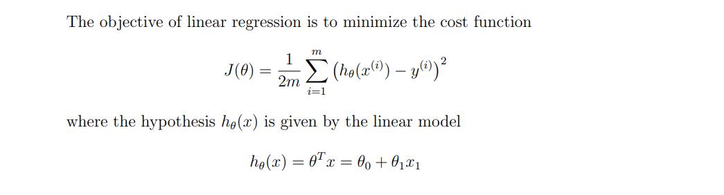
上述两个公式就是这章的重点了。

一个就是我们的模型预测函数h(x)。
我们要做的就是不断去迭代更新两个theta的值以做到让这个均值平方差(损失)最小，最后就是去拿这一对最优解去进行后续的预测。

梯度下降法

我们在上面提到了迭代更新，吴老师在视频中讲述了ML的第一个算法，梯度下降法。梯度就是slope，其实简而言之就是我们的导数。我们知道沿导数方向可以做到最快的下降。

这里还有几个注意点
1.梯度下降法有时候会陷入局部最优解从而漏掉全局最优解。
2.从不同位置进行梯度下降法可能得到的解不同。但是！基于我们优化的代价函数是convex凸函数，总是可以得到最优解。

求导，不具体推导了，同济大学的绿不拉机的书伺候。

其实就是换元咯，把(h(x) - y)视为t， 最后就是2t × h(x)对theta求偏导。
这里的alpha我们称之为学习率。

学习率太小则需要多轮迭代。
学习率太大则有可能错过最优解，甚至离其越来越远。

线性代数

矩阵与向量。
矩阵向量乘法。
矩阵乘法。
矩阵的转置和逆。

课后作业

作业自己得去网上找资源哈，git上有，我忘了链接了。。。。

1.了解一些基本的编程语法。跳过具体步骤，以创建一个对角1矩阵为例。
这里换成numpy来生成也可以。

def function1():
    # helps you be familiar with the python syntax
    x = torch.eye(5, dtype=torch.int)
    print(x)

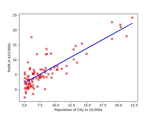
2.从ex1的txt文件中读取数据，并画出散点图。

def function2():
    # linear regression with only one Variable
    # you will be demand to predict the profit for a food truck and the dataset is in 'ex1.txt'
    # first you should plot a scatter picture
    file = pd.read_csv("./ex1data1.txt", header=None, names=["Population", "Profit"])
    # print(file)
    x_set = file["Population"]
    y_set = file["Profit"]
    plt.scatter(x_set, y_set, marker='x', c='red')
    plt.ylabel("Profit in $10,000s", loc="center")
    plt.xlabel("Population of City in 10,000s", loc="center")
    plt.show()

对csv文件理解还是要深刻一些，它其实是逗号分割符文件。这样一来用pandas读再转array会很方便。比直接用open配合readline来实现要好很多。
结果图：

3.完成损失函数的设计，然后进行梯度下降法的实现。
打印每一轮的损失值，最后实现可视化。

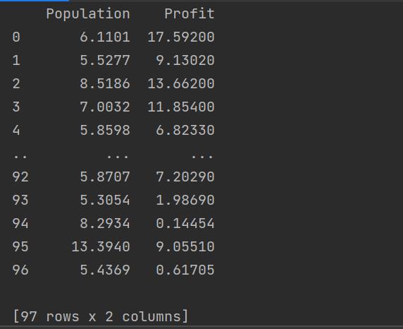
注意：题目中吴老师要求我们做单变量(这里的Population就是我们的唯一变量)的梯度下降，他题目中补充的一种思路就是在原先的Populations前边加上一列全1用以代表theta0相乘的值，也就是视为
hx = theta0 × 1 + theta1 × X。

我们的file变量是一个Dataframe，样子如下：

我们对下面的代码略微解读：
theta0就是我们的全一列，我们用colomn_stack来进行堆叠。就是按列堆叠，简单理解就是把theta0这个全一视为一列堆到M矩阵的左边去。
这个M就是我们直接由file利用numpy转换过来的一个array类型。

numpy实际上还有matrix矩阵类型可以用，用在这里实际上会更加方便。
因为我们知道矩阵相称的规则就是做矩阵的列数要和右矩阵的行数相等。
我会在(4)中加以操作。

这里sub变量就是中间的差值，可以看到我们需要用dot函数才可以对array类型进行矩阵一样的运算。而如果这里面的变量都是matrix的话，直接用乘号即可。

最后就是里面众多的reshape(-1,1)就是转化为[N，1]的矩阵。否则单取一列的话你的shape是(N, )第二个维度是空的说明这个实际上是一个向量。这样在进行运算时会有很多bug出现。

以上是我觉得一些困难的点，具体的就由自己下载好作业文件，把txt复制到和你的python同一目录下，然后debug执行。
多看看array的shape，你就会明白代码里一些看似多余的操作。你可以删去你认为的多余的操作看看有什么exception出现。

def function3():
    """
    In this part, you will fit the linear regression parameters θ to our dataset
    using gradient descent.
    """
    file = pd.read_csv("./ex1data1.txt", header=None, names=["Population", "Profit"])
    # print(file)
    M = np.array(file)
    length = len(M[:, 1])
    theta0 = np.ones((length, 1))
    M = np.column_stack((theta0, M))
    theta = np.zeros((2, 1))

    # print(theta)
    iterations = 1500
    learning_rate = 0.01
    reals = M[:, 2].reshape(-1, 1)  # 扩维 否则只是一个向量没法计算
    x_coef = M[:, 1].reshape(-1, 1)
    # print(theta[0, 0], theta[1, 0])
    for i in range(iterations):
        loss = 0
        sub = np.dot(M[:, :-1], theta) - reals
        loss += np.sum(np.power(sub, 2) / (2 * length))
        print("loss is %f" % loss)
        temp = theta
        for j in range(2):
            yy = sub * M[:, j].reshape(-1, 1)
            temp[j, 0] = theta[j, 0] - learning_rate * 1 / length * np.sum(yy)
        theta = temp
    x_set = np.array(file["Population"])
    y_set = np.array(file["Profit"])
    predicts = np.dot(M[:, :-1], theta)
    plt.plot(x_set, predicts, color="blue")
    plt.scatter(x_set, y_set, marker='x', c='red')
    plt.ylabel("Profit in $10,000s", loc="center")
    plt.xlabel("Population of City in 10,000s", loc="center")
    plt.show()

最后的拟合结果图。

4.多元梯度下降法和正规方程法。
多元梯度下降法其实也是比较容易的，甚至代码和单变量的相比是无需任何改变的。我们会把模型函数进行一个扩充：
h(x) = theta0 + theta1 * X1 + theta2 * X2 + … + thetan * Xn
但无论如何我们都是可以视为矩阵相乘的形式的。
我们的optional exercise说明了，ex2.txt文件就是一个多变量文件。

同样地我们把文件读入后的结果做一个展示：
可以看到其实也只有两个变量而已。。。

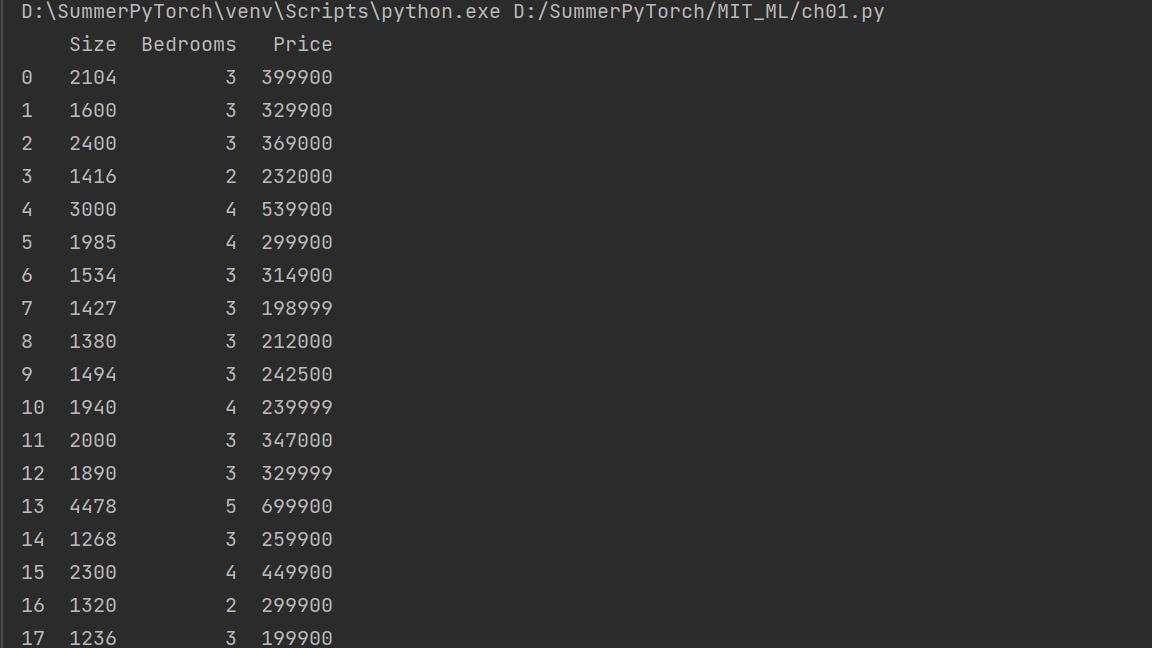
归一化，特征缩放，feature scaling。
就是说，你的特征的取值范围相似时会更快地收敛。像刚刚的ex2文件的特征直接用于回归法就不是一个明智的选择，会需要很多轮迭代才可以，甚至有可能因为值太大而导致溢出。
所以我们事先会为特征做一个归一化处理：

 file = pd.read_csv("./ex1data2.txt", header=None, names=["Size", "Bedrooms", "Price"])
    # print(file)
    size = len(file["Size"])
    X = np.matrix(np.ones((size, 3)))    # 这样一来等会就把提取出来的两列进行一个填充即可，第一列全1就无需再补
    x_size, x_bedroom = np.array(file["Size"]).reshape(-1, 1), np.array(file["Bedrooms"]).reshape(-1, 1)
    x_size = x_size / np.max(x_size)
    x_bedroom = x_bedroom / np.max(x_bedroom)
    X[:, 1] = x_size
    X[:, 2] = x_bedroom

上面的代码中我们是事先创造一个全一矩阵然后进行填充处理。

我们先来试一试基于梯度下降法的多元回归实现。
我得到的 损失&迭代次数 图形如下：

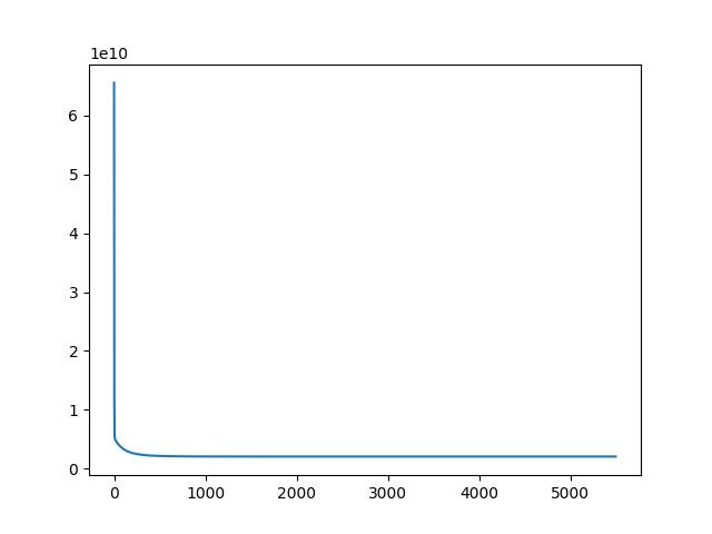
千万别看后面已经很平了，注意纵坐标要乘上le10，一点点下降都是很夸张的！

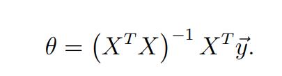
正规方程法：
这里并不想用线性代数&高数的知识来推导，可以去找一些优秀的blog进行学习。
这里直接给出公式：
X就是我们的特征矩阵，y是我们的labels向量，就是我们要预测的那个值。

最后给出两种方法的损失差别：
不难看出，梯度下降仍旧是没有完全收敛，有兴趣和时间的话可以自己调整参数（learning_rate + iterations）做到和正规方程法完全一致。

完整代码：

import torch
import numpy as np
import pandas as pd
import matplotlib.pyplot as plt
from mpl_toolkits.mplot3d import Axes3D

'''
In this exercise, you will implement linear regression and get to see it work
on data. Before starting on this programming exercise, we strongly 
recommend watching the video lectures and completing the review questions for
the associated topics.
'''


def syntax():
    # helps you be familiar with the python syntax
    x = torch.eye(5, dtype=torch.int)
    print(x)


def read_txt_2_Dataframe():
    # linear regression with only one Variable
    # you will be demand to predict the profit for a food truck and the dataset is in 'ex1.txt'
    # first you should plot a scatter picture
    file = pd.read_csv("./ex1data1.txt", header=None, names=["Population", "Profit"])
    print(file)
    x_set = file["Population"]
    y_set = file["Profit"]
    plt.scatter(x_set, y_set, marker='x', c='red')
    plt.ylabel("Profit in $10,000s", loc="center")
    plt.xlabel("Population of City in 10,000s", loc="center")
    plt.show()


def draw_loss_J_theta(x, y, z):
    x = np.array(x)
    y = np.array(y)
    z = np.array(z).reshape(-1, 1)
    fig = plt.figure()
    # ax = Axes3D(fig)
    ax = fig.add_subplot(111, projection='3d')
    ax.plot_surface(x, y, z, rstride=1, cstride=1, cmap=plt.get_cmap('rainbow'))

    plt.show()


def one_variable_linear_regression():
    """
    In this part, you will fit the linear regression parameters θ to our dataset
    using gradient descent.
    """
    file = pd.read_csv("./ex1data1.txt", header=None, names=["Population", "Profit"])
    # print(file)
    M = np.array(file)
    length = len(M[:, 1])
    theta0 = np.ones((length, 1))
    M = np.column_stack((theta0, M))
    theta = np.zeros((2, 1))

    theta_0 = []
    theta_1 = []
    loss_list = []

    # print(theta)
    iterations = 1500
    learning_rate = 0.01
    reals = M[:, 2].reshape(-1, 1)  # 扩维 否则只是一个向量没法计算
    x_coef = M[:, 1].reshape(-1, 1)
    # print(theta[0, 0], theta[1, 0])
    for i in range(iterations):
        loss = 0
        sub = np.dot(M[:, :-1], theta) - reals
        loss += np.sum(np.power(sub, 2) / (2 * length))
        theta_0.append(theta[0, 0])
        theta_1.append(theta[1, 0])
        loss_list.append(loss)
        print("loss is %f" % loss)
        for j in range(2):
            yy = sub * M[:, j].reshape(-1, 1)
            theta[j, 0] = theta[j, 0] - learning_rate * 1 / length * np.sum(yy)
    x_set = np.array(file["Population"])
    y_set = np.array(file["Profit"])
    predicts = np.dot(M[:, :-1], theta)
    plt.plot(x_set, predicts, color="blue")
    plt.scatter(x_set, y_set, marker='x', c='red')
    plt.ylabel("Profit in $10,000s", loc="center")
    plt.xlabel("Population of City in 10,000s", loc="center")
    plt.show()

    # draw_loss_J_theta(theta_0, theta_1, loss_list)


def multi_variable_linear_regression_equation_method():
    # file = pd.read_csv("./ex1data1.txt", header=None, names=["Population", "Profit"])
    file = pd.read_csv("./ex1data2.txt", header=None, names=["Size", "Bedrooms", "Price"])
    # print(file)
    size = len(file["Size"])
    X = np.matrix(np.ones((size, 3)))    # 这样一来等会就把提取出来的两列进行一个填充即可，第一列全1就无需再补
    x_size, x_bedroom = np.array(file["Size"]).reshape(-1, 1), np.array(file["Bedrooms"]).reshape(-1, 1)
    x_size = x_size / np.max(x_size)
    x_bedroom = x_bedroom / np.max(x_bedroom)
    X[:, 1] = x_size
    X[:, 2] = x_bedroom
    labels = np.matrix(np.array(file["Price"]).reshape(-1, 1))
    theta = np.matrix(np.zeros((3, 1)))  # 系数一开始都是初始化为0
    iterations = 5500
    learning_rate = 0.20
    loss_list = []
    iter_list = []
    for i in range(iterations):
        iter_list.append(i)
        sub = X * theta - labels
        loss = np.sum(np.power(sub, 2) / (2 * size))
        loss_list.append(loss)
        for j in range(3):
            sub_arr = np.array(sub)
            yy = sub_arr * np.array(X[:, j])
            theta[j, 0] = theta[j, 0] - np.sum(yy) * learning_rate * 1 / size
    plt.plot(iter_list, loss_list)
    plt.show()
    print("Gradient Descent : %f" % loss)
    temp = theta.copy()
    """
    we use equations to calculate the best theta directly
    if we have millions of records then it's better to use gradient descend method
    On the other hand, if the matrix is not invertible, we can't use equation method
    """
    theta = np.linalg.inv(np.transpose(X) * X) * np.transpose(X) * labels
    sub = X * theta - labels
    loss = np.sum(np.power(sub, 2) / (2 * size))
    print("Equation : %f" % loss)


if __name__ == "__main__":
    # one_variable_linear_regression()
    multi_variable_linear_regression_equation_method()