数据科学项目02：NLP应用之垃圾短信/邮件检测（端到端的项目）

Posted 2022-08-26 JOJO数据科学

tags:

篇首语：本文由小常识网(cha138.com)小编为大家整理，主要介绍了数据科学项目02：NLP应用之垃圾短信/邮件检测（端到端的项目）相关的知识，希望对你有一定的参考价值。

垃圾短信检测（端到端的项目）

我们都听说过一个流行词——“数据科学”。我们大多数人都对“它是什么？我可以成为数据分析师或数据科学家吗？我需要什么技能？并不是很了解。例如：我想开始一个数据科学项目，但我却不知道如何着手进行。
我们大多数人都是通过一些在线课程了解了这个领域。我们对课程中布置的作业和项目感到游刃有余。但是，当开始分析全新或未知的数据集时，我们会迷失方向。为了在分析我们遇到的任何数据集和问题时，我们需要通过不断的练习。我觉得最好的方式之一就是在项目中进行学习。所以每个人都需要开始自己的第一个项目。因此，我准备写一个专栏，带大家一起完成数据科学项目，感兴趣的朋友可以一起交流学习。本专栏是一个以实战为主的专栏。

0.引言

随着产品和服务在线消费的增加，消费者面临着收件箱中大量垃圾邮件的巨大问题，这些垃圾邮件要么是基于促销的，要么是欺诈性的。由于这个原因，一些非常重要的消息/电子邮件被当做垃圾短信处理了。在本文中，我们将创建一个垃圾短信/邮件检测模型，该模型将使用朴素贝叶斯和自然语言处理(NLP) 来确定是否为垃圾短信/邮件。

在这里我使用的是colab内置环境，完整代码文末获取。

额外的所需包如下，大家自行安装

nltk
streamlit
pickle

1.数据收集和加载

我们将使用kaggle提供的数据集：数据集

该数据集包含一组带有标记的短信文本，这些消息被归类为正常短信和垃圾短信。 每行包含一条消息。每行由两列组成：v1 带有标签，（spam 或 ham），v2 是文本内容。

df=pd.read_csv('/content/spam/spam.csv',encoding='latin-1')#这里encoding需要指定为latin-1

# 查看一下数据基本情况
df.head()

	v1	v2	Unnamed: 2	Unnamed: 3	Unnamed: 4
0	ham	Go until jurong point, crazy.. Available only ...	NaN	NaN	NaN
1	ham	Ok lar... Joking wif u oni...	NaN	NaN	NaN
2	spam	Free entry in 2 a wkly comp to win FA Cup fina...	NaN	NaN	NaN
3	ham	U dun say so early hor... U c already then say...	NaN	NaN	NaN
4	ham	Nah I don't think he goes to usf, he lives aro...	NaN	NaN	NaN

该数据包含一组带有标记的短信数据，其中：

v1表示短信标签，ham表示正常信息，spam表示垃圾信息
v2是短信的内容

#去除不需要的列
df=df.iloc[:,:2]

#重命名列
df=df.rename(columns="v1":"label","v2":"message")
df.head()

	label	message
0	ham	Go until jurong point, crazy.. Available only ...
1	ham	Ok lar... Joking wif u oni...
2	spam	Free entry in 2 a wkly comp to win FA Cup fina...
3	ham	U dun say so early hor... U c already then say...
4	ham	Nah I don't think he goes to usf, he lives aro...

# 将lable进行one-hot编码，其中0:ham，1:spam
from sklearn.preprocessing import LabelEncoder
encoder = LabelEncoder()

df['label']=encoder.fit_transform(df['label'])
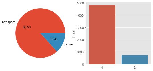
df['label'].value_counts()

0    4825
1     747
Name: label, dtype: int64

可以看出一共有747个垃圾短信

# 查看缺失值
df.isnull().sum()
# 数据没有缺失值

label      0
message    0
dtype: int64

2.探索性数据分析（EDA）

通过可视化分析来更好的理解数据

import matplotlib.pyplot as plt
plt.style.use('ggplot')
plt.figure(figsize=(9,4))
plt.subplot(1,2,1)
plt.pie(df['label'].value_counts(),labels=['not spam','spam'],autopct="%0.2f")
plt.subplot(1,2,2)
sns.barplot(x=df['label'].value_counts().index,y=df['label'].value_counts(),data=df)
plt.show()

在特征工程部分，我简单创建了一些单独的特征来提取信息

字符数
单词数
句子数

#1.字符数
df['char']=df['message'].apply(len)

nltk.download('punkt')

[nltk_data] Downloading package punkt to /root/nltk_data...
[nltk_data]   Unzipping tokenizers/punkt.zip.

True

#2.单词数,这里我们首先要对其进行分词处理，使用nltk
#分词处理
df['words']=df['message'].apply(lambda x: len(nltk.word_tokenize(x)))

# 3.句子数
df['sen']=df['message'].apply(lambda x: len(nltk.sent_tokenize(x)))

df.head()

	label	message	char	words	sen
0	0	Go until jurong point, crazy.. Available only ...	111	24	2
1	0	Ok lar... Joking wif u oni...	29	8	2
2	1	Free entry in 2 a wkly comp to win FA Cup fina...	155	37	2
3	0	U dun say so early hor... U c already then say...	49	13	1
4	0	Nah I don't think he goes to usf, he lives aro...	61	15	1

描述性统计

# 描述性统计
df.describe()

index	label	char	words	sen
count	5572.0	5572.0	5572.0	5572.0
mean	0.13406317300789664	80.11880832735105	18.69562096195262	1.9707465900933239
std	0.34075075489776974	59.6908407765033	13.742586801744975	1.4177777134026657
min	0.0	2.0	1.0	1.0
25%	0.0	36.0	9.0	1.0
50%	0.0	61.0	15.0	1.0
75%	0.0	121.0	27.0	2.0
max	1.0	910.0	220.0	28.0

下面我们通过可视化比较一下不同短信在这些数字特征上的分布情况

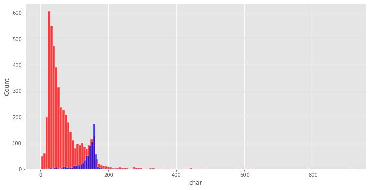
# 字符数比较
plt.figure(figsize=(12,6))
sns.histplot(df[df['label']==0]['char'],color='red')#正常短信
sns.histplot(df[df['label']==1]['char'],color = 'blue')#垃圾短信

<matplotlib.axes._subplots.AxesSubplot at 0x7fce63763dd0>

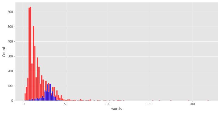
# 比较
plt.figure(figsize=(12,6))
sns.histplot(df[df['label']==0]['words'],color='red')#正常短信
sns.histplot(df[df['label']==1]['words'],color = 'blue')#垃圾短信

<matplotlib.axes._subplots.AxesSubplot at 0x7fce63f4bed0>

sns.pairplot(df,hue='label')

#删除数据集中存在的一些异常值
i=df[df['char']>500].index
df.drop(i,axis=0,inplace=True)

df=df.reset_index()
df.drop("index",inplace=True,axis=1)

#相关系数矩阵
sns.heatmap(df.corr(),annot=True)

<matplotlib.axes._subplots.AxesSubplot at 0x7fce606d0250>

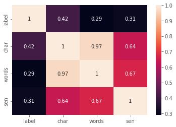
我们这里看到存在多重共线性，因此，我们不使用所有的列，在这里选择与label相关性最强的char

3.数据预处理

对于英文文本数据，我们常用的数据预处理方式如下

去除标点符号
去除停用词
去除专有名词
变换成小写
分词处理
词根、词缀处理

下面我们来看看如何实现这些步骤

nltk.download('stopwords')

[nltk_data] Downloading package stopwords to /root/nltk_data...
[nltk_data]   Unzipping corpora/stopwords.zip.

True

# 首先导入需要使用到的包
from nltk.corpus import stopwords
from nltk.stem import PorterStemmer
from wordcloud import WordCloud
import string,time

# 标点符号
string.punctuation

'!"#$%&\\'()*+,-./:;<=>?@[\\\\]^_`|~'

# 停用词
stopwords.words('english')

3.1清洗文本数据

去除web链接
去除邮件
取掉数字

下面使用正则表达式来处理这些数据。

def remove_website_links(text):
    no_website_links = text.replace(r"http\\S+", "")#去除网络连接
    return no_website_links

def remove_numbers(text):
    removed_numbers = text.replace(r'\\d+','')#去除数字
    return removed_numbers

def remove_emails(text):
    no_emails = text.replace(r"\\S*@\\S*\\s?",'')#去除邮件
    return no_emails

df['message'] = df['message'].apply(remove_website_links)
df['message'] = df['message'].apply(remove_numbers)
df['message'] = df['message'].apply(remove_emails)

df.head()

	label	message	char	words	sen
0	0	Go until jurong point, crazy.. Available only ...	111	24	2
1	0	Ok lar... Joking wif u oni...	29	8	2
2	1	Free entry in 2 a wkly comp to win FA Cup fina...	155	37	2
3	0	U dun say so early hor... U c already then say...	49	13	1
4	0	Nah I don't think he goes to usf, he lives aro...	61	15	1

3.2 文本特征转换

def message_transform(text):
  
  text = text.lower()#转换为小写
  
  text = nltk.word_tokenize(text)#分词处理
  
  # 去除停用词和标点
  y = []#创建一个空列表
  for word in text:
    stopwords_punc = stopwords.words('english')+list(string.punctuation)#存放停用词和标点
    if word.isalnum()==True and word not in stopwords_punc:
      y.append(word)
  
  # 词根变换
  message=y[:]
  y.clear()
  for i in message:
    ps=PorterStemmer()
    y.append(ps.stem(i))
  return " ".join(y)#返回字符串形式

df['message'] = df['message'].apply(message_transform)
df['num_words_transform']=df['message'].apply(lambda x: len(str(x).split()))

df.head()

	label	message	char	words	sen
0	0	Go until jurong point, crazy.. Available only ...	111	24	2
1	0	Ok lar... Joking wif u oni...	29	8	2
2	1	Free entry in 2 a wkly comp to win FA Cup fina...	155	37	2
3	0	U dun say so early hor... U c already then say...	49	13	1
4	0	Nah I don't think he goes to usf, he lives aro...	61	15	1

4.词频统计

4.1绘制词云

#绘制信息中出现最多的词的词云
from wordcloud import WordCloud
#首先，创建一个object
wc=WordCloud(width=500,height=500,min_font_size=10,background_color='white')

# 垃圾信息的词云
spam_wc=wc.generate(df[df['label']==1]['message'].str.cat(sep=""))

plt.figure(figsize=(18,12))
plt.imshow(spam_wc)

<matplotlib.image.AxesImage at 0x7fce5d938710>

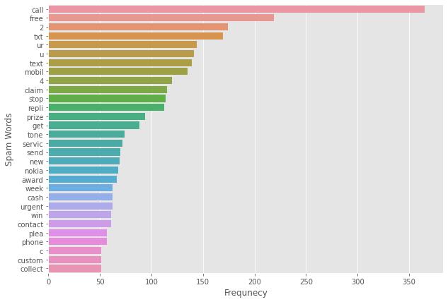
可以看出，这些垃圾邮件出现频次最多的单词是：free、call等这种具有诱导性的信息

# 正常信息的词云
ham_wc = wc.generate(df[df['label']==0]['message'].str.cat(sep=''))
plt.figure(figsize=(18,12))
plt.imshow(ham_wc)

<matplotlib.image.AxesImage at 0x7fce607af190>

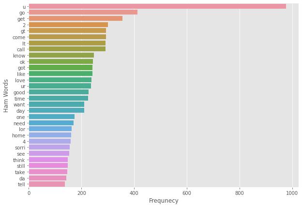
可以看出正常信息出现频次较多的单词为u、go、got、want等一些传达信息的单词

为了简化词云图的信息，我们现在分别统计垃圾短信和正常短信频次top30的单词

4.2找出词数top30的单词

垃圾短信：

# 统计词频
spam_corpus=[]
for i in df[df['label']==1]['message'].tolist():
  for word in i.split():
        spam_corpus.append(word)

from collections import Counter
Counter(spam_corpus)#记数
Counter(spam_corpus).most_common(30)#取最多的30个单词
plt.figure(figsize=(10,7))
sns.barplot(y=pd.DataFrame(Counter(spam_corpus).most_common(30))[0],x=pd.DataFrame(Counter(spam_corpus).most_common(30))[1])
plt.xticks()
plt.xlabel("Frequnecy")
plt.ylabel("Spam Words")
plt.show()

正常短信

ham_corpus=[]
for i in df[df['label']==0]['message'].tolist():
  for word in i.split():
    ham_corpus.append(word)

from collections import Counter
plt.figure(figsize=(10,7))
sns.barplot(y=pd.DataFrame(Counter(ham_corpus).most_common(30))[0],x=pd.DataFrame(Counter(ham_corpus).most_common(30))[1])
plt.xticks()
plt.xlabel("Frequnecy")
plt.ylabel("Ham Words")
plt.show()

下面进一步分析垃圾短信和非垃圾短信的单词和字符数分布情况

# 字符数
fig,(ax1,ax2)=plt.subplots(1,2,figsize=(15,6))
text_len=df[df['label']==1]['text'].str.len()
ax1.hist(text_len,color='green')
ax1.set_title('Original text')
text_len=df[df['label']==0]['text'].str.len()
ax2.hist(text_len,color='red')
ax2.set_title('Fake text')
fig.suptitle('Characters in texts')
plt.show()

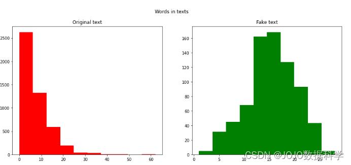
#单词数
fig,(ax1,ax2)=plt.subplots(1,2,figsize=(15,6))
text_len=df[df['label']==1]['num_words_transform']
ax1.hist(text_len,color='red')
ax1.set_title('Original text')
text_len=df[df['label']==0]['num_words_transform']
ax2.hist(text_len,color='green')
ax2.set_title('Fake text')
fig.suptitle('Words in texts')
plt.show()

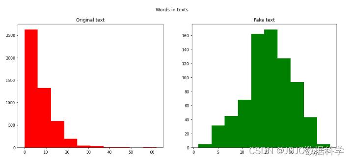
总结
经过上面分析，我们可以得出结论，垃圾短信文本与非垃圾短信文本相比具有更多的单词和字符。

垃圾短信中包含的平均字符数约为 90 个字符
垃圾短信中包含的平均字数约为 15 个字

5.模型构建

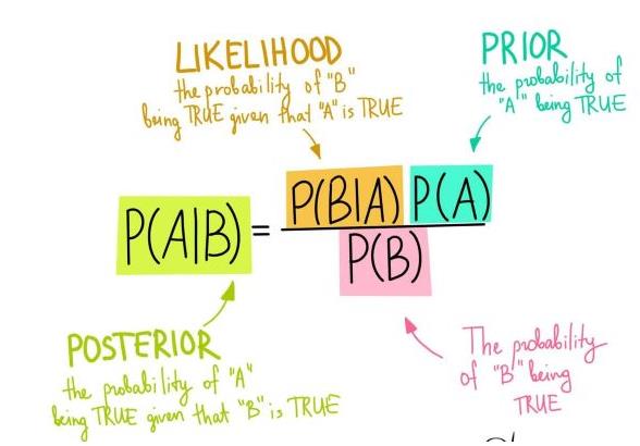
根据历史经验，在文本数据上朴素贝叶斯算法效果很好，因此我们将使用它，但在此过程中还将它与不同的算法进行比较。
在统计学中，朴素贝叶斯分类器是一系列简单的“概率分类器”，它们基于应用贝叶斯定理和特征之间的（朴素）条件独立假设。它们是最简单的贝叶斯网络模型之一，但与核密度估计相结合，它们可以达到更高的准确度水平。

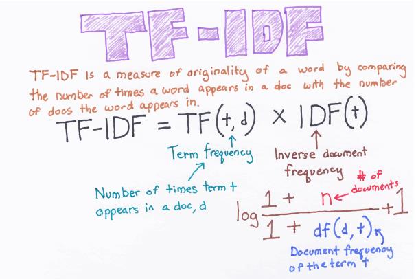
首先，我们这里的输入数据是文本数据，不能够直接建立模型。因此，我们必须将这些文本数据进行特征提取。比较常用的几种方法：

词袋模型（Bag of words） 存在稀疏性问题
TF-IDF
Word2vec

因为是实战训练，在这里不具体展开的几种方法的原理，在这里我选择TF-IDF。

我也试了一下Word embedding，结合一些深度学习的方法，精度能够有所提高，感兴趣的小伙伴可以自己尝试一下，基本步骤类似。下面我们首先建立贝叶斯模型。

5.1 构建贝叶斯模型

from sklearn.feature_extraction.text import TfidfVectorizer
tfidf = TfidfVectorizer(max_features=3000)

X = tfidf.fit_transform(df['message']).toarray()
y = df['label'].values

array([0, 0, 1, ..., 0, 0, 0])

from sklearn.model_selection import train_test_split
X_train,X_test,y_train,y_test = train_test_split(X,y,test_size=0.2,random_state=2)#训练集测试集划分

from sklearn.naive_bayes import GaussianNB,MultinomialNB,BernoulliNB
from sklearn.metrics import accuracy_score,confusion_matrix,precision_score

这里我们比较三种不同的贝叶斯模型的各个评估指标结果

#GaussianNB
gnb = GaussianNB()
gnb.fit(X_train,y_train)
y_pred1 = gnb.predict(X_test)
print("Accuracy Score -",accuracy_score(y_test,y_pred1))
print("Precision Score -",precision_score(y_test,y_pred1))
print(confusion_matrix(y_test,y_pred1))

Accuracy Score - 0.8456014362657092
Precision Score - 0.47038327526132406
[[807 152]
 [ 20 135]]

#MultinomialNB
mnb = MultinomialNB()
mnb.fit(X_train,y_train)
y_pred2 = mnb.predict(X_test)
print("Accuracy Score -",accuracy_score(y_test,y_pred2))
print("Precision Score -",precision_score(y_test,y_pred2))
print(confusion_matrix(y_test,y_pred2))

Accuracy Score - 0.9793536804308797
Precision Score - 0.9925373134328358

[[958   1]
 [ 22 133]]

#Bernuli
bnb = BernoulliNB()
bnb.fit(X_train,y_train)
y_pred3 = bnb.predict(X_test)
print垃圾短信邮件判断算法
 目前最好的垃圾邮件过滤算法
 分类算法之决策树
 用于电子邮件垃圾邮件检测的神经网络输入
 朴素贝叶斯分类之垃圾短信识别
 基于卷积神经网络(CNN)的中文垃圾邮件检测