优化算法多目标花朵授粉算法（MOFPA）含Matlab源码 1594期

Posted 2022-01-03 紫极神光

一、获取代码方式

获取代码方式1：
完整代码已上传我的资源：【优化算法】多目标花朵授粉算法（MOFPA）【含Matlab源码 1594期】

获取代码方式2：
通过订阅紫极神光博客付费专栏，凭支付凭证，私信博主，可获得此代码。

备注：
订阅紫极神光博客付费专栏，可免费获得1份代码（有效期为订阅日起，三天内有效）；

二、花朵授粉算法简介

介绍了一种新的元启发式群智能算法——花朵授粉算法（flower pollinate algorithm，FPA）和一种新型的差分进化变异策略——定向变异（targeted mutation，TM）策略。针对FPA存在的收敛速度慢、寻优精度低、易陷入局部最优等问题，提出了一种基于变异策略的改进型花朵授粉算法——MFPA。该算法通过改进TM策略，并应用到FPA的局部搜索过程中，以增强算法的局部开发能力。

三、部分源代码

% --------------------------------------------------------------------    % 
% Multiobjective flower pollenation algorithm (MOFPA)                     %

%%%%%%%%%%%%%%%%%%%%%%%%%%%%%%%%%%%%%%%%%%%%%%%%%%%%%%%%%%%%%%%%%%%%%%%%%%%
% Notes: This demo program contains the very basic components of          %
% the multiobjective flower pollination algorithm (MOFPA)                 % 
% for bi-objective optimization. It usually works well for                %
% unconstrained functions only. For functions/problems with               % 
% limits/bounds and constraints, constraint-handling techniques           %
% should be implemented to deal with constrained problems properly.       %
%                                                                         %   


%% Notes: --------------------------------------------------------------- %
% n=# of the solutions in the population
% m=# of objectives, d=# of dimensions
% S or Sol has a size of n by d
% f = objective values of [n by m]
% RnD = Rank of solutions and crowding Distances, so size of [n by 2]    %

function [best,fmin,N_iter]=mofpa(para)
% Default parameters
if nargin<1,
   para=[100 1000 0.8];
end
n=para(1);           % Population size, typically 10 to 25
Iter_max=para(2);    % Max number of iterations
p=para(3);           % probabibility switch

% Number of objectives
m=2;
% Rank and distance matrix
RnD=zeros(n,2);
% Dimension of the search variables
d=30;
% Simple lower and upper bounds
Lb=0*ones(1,d);    Ub=1*ones(1,d);

%% Initialize the population
for i=1:n,
   Sol(i,:)=Lb+(Ub-Lb).*rand(1,d); 
   f(i,1:m) = obj_funs(Sol(i,:), m);
end
% Store the fitness or objective values
f_new=f;
%% Sort the initialized population
x=[Sol f];  % combined into a single input
% Non-dominated sorting for the initila population
Sorted=solutions_sorting(x, m,d);
% Decompose into solutions, fitness, rank and distances
Sol=Sorted(:,1:d);
f=Sorted(:,(d+1):(d+m));
RnD=Sorted(:,(d+m+1):end);

% Start the iterations -- Flower Algorithm 
for t=1:Iter_max,
        % Loop over all flowers/solutions
        for i=1:n,
          % Pollens are carried by insects and thus can move in
          % large scale, large distance.
          % This L should replace by Levy flights  
          % Formula: x_i^t+1=x_i^t+ L (x_i^t-gbest)
          if rand>p,
          %% L=rand;
          L=Levy(d);     
    % The best is stored as the first row Sol(1,:) of the sorted solutions 
          dS=L.*(Sol(i,:)-Sol(1,:));
          S(i,:)=Sol(i,:)+dS;
  
          % Check if the simple limits/bounds are OK
          S(i,:)=simplebounds(S(i,:),Lb,Ub);
          
          % If not, then local pollenation of neighbor flowers 
          else
              epsilon=rand;
              % Find random flowers in the neighbourhood
              JK=randperm(n);
              % As they are random, the first two entries also random
              % If the flower are the same or similar species, then
              % they can be pollenated, otherwise, no action.
              % Formula: x_i^t+1+epsilon*(x_j^t-x_k^t)
              S(i,:)=Sol(1,:)+epsilon*(Sol(JK(1),:)-Sol(JK(2),:));
              % Check if the simple limits/bounds are OK
              S(i,:)=simplebounds(S(i,:),Lb,Ub);
          end
        end % end of for loop
        
      
   %% Evalute the fitness/function values of the new population
   for i=1:n,
        f_new(i, 1:m) = obj_funs(S(i,1:d),m);
     
        if (f_new(i,1:m) <= f(i,1:m)),  
            f(i,1:m)=f_new(i,1:m);
        end
        % Update the current best (stored in the first row)
        if (f_new(i,1:m) <= f(1,1:m)), 
            Sol(1,1:d) = S(i,1:d); 
            f(1,:)=f_new(i,:);
        end
        
     end % end of for loop

%% ! It's very important to combine both populations, otherwise,
%% the results may look odd and will be very inefficient. !     
%% The combined population consits of both the old and new solutions
%% So the total size of the combined population for sorting is 2*n
       X(1:n,:)=[S f_new];            % Combine new solutions
       X((n+1):(2*n),:)=[Sol f];      % Combine old solutions
       Sorted=solutions_sorting(X, m, d);
       %% Select n solutions among a combined population of 2*n solutions
       new_Sol=Select_pop(Sorted, m, d, n);
       % Decompose into solutions, fitness and ranking
       Sol=new_Sol(:,1:d);             % Sorted solutions
       f=new_Sol(:,(d+1):(d+m));       % Sorted objective values
       RnD=new_Sol(:,(d+m+1):end);     % Sorted ranks and distances
    
  %% Running display at each 100 iterations
   if ~mod(t,100), 
     disp(strcat('Iterations t=',num2str(t))); 
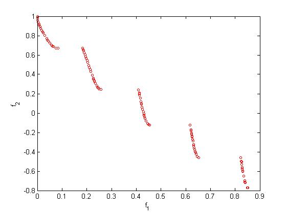
     plot(f(:, 1), f(:, 2),'ro','MarkerSize',3); 
     % axis([0 1 -0.8 1]);
     xlabel('f_1'); ylabel('f_2');
     drawnow;
   end   
     
end  % end of iterations

%% End of the main program %%%%%%%%%%%%%%%%%%%%%%%%%%%%%%%%%%%%%%%%%%%%%%%%

% Application of simple constraints or bounds
function s=simplebounds(s,Lb,Ub)
  % Apply the lower bound
  ns_tmp=s;
  I=ns_tmp<Lb;
  ns_tmp(I)=Lb(I);
  
  % Apply the upper bounds 
  J=ns_tmp>Ub;
  ns_tmp(J)=Ub(J);
  % Update this new move 
  s=ns_tmp;

% Draw n Levy flight sample
function L=Levy(d)
% Levy exponent and coefficient
% For details, see Chapter 11 of the following book:
% Xin-She Yang, Nature-Inspired Optimization Algorithms, Elsevier, (2014).
beta=3/2;
sigma=(gamma(1+beta)*sin(pi*beta/2)/(gamma((1+beta)/2)*beta*2^((beta-1)/2)))^(1/beta);
    u=randn(1,d)*sigma;
    v=randn(1,d);
    step=u./abs(v).^(1/beta);
L=0.1*step; 

%%%%%%%%%%%%%%%%%%%%%%%%%%%%%%%%%%%%%%%%%%%%%%%%%%%%%%%%%%%%%%%%%%%%%%%%%%%
% Make sure all the new solutions are within the limits
function [ns]=findlimits(ns,Lb,Ub)
  % Apply the lower bound
  ns_tmp=ns;
  I=ns_tmp < Lb;
  ns_tmp(I)=Lb(I);
  
  % Apply the upper bounds 
  J=ns_tmp>Ub;
  ns_tmp(J)=Ub(J);
  % Update this new move 
  ns=ns_tmp;

四、运行结果

五、matlab版本及参考文献

1 matlab版本
2014a

2 参考文献
[1] 包子阳,余继周,杨杉.智能优化算法及其MATLAB实例（第2版）[M].电子工业出版社，2016.
[2]张岩,吴水根.MATLAB优化算法源代码[M].清华大学出版社，2017.