优化算法迭代扩展卡尔曼滤波算法（IEKF）含Matlab源码 1584期

Posted 2022-01-03 紫极神光

一、获取代码方式

获取代码方式1：
通过订阅紫极神光博客付费专栏，凭支付凭证，私信博主，可获得此代码。

获取代码方式2：
完整代码已上传我的资源：【优化算法】迭代扩展卡尔曼滤波算法（IEKF）【含Matlab源码 1584期】

备注：
订阅紫极神光博客付费专栏，可免费获得1份代码（有效期为订阅日起，三天内有效）；

二、迭代扩展卡尔曼滤波算法（IEKF）简介

IEKF与EKF的不同之处主要在于测量更新过程，对于IEKF, 在得到状态预测


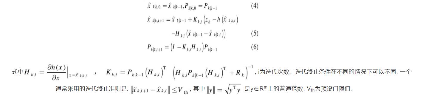
文献[8]证明了IEKF迭代结果与高斯牛顿方法估计的结果是一致的, 因此IEKF可以保证全局收敛。理论上, IEKF优于EKF和MVEKF, 然而, 实际中并不完全如此, 因为: (1) 文献[8]给出的结论是建立在必须满足局部线性化条件的假设之上, 也就是说, 状态估计必须足够接近于真实值, 这在很多应用中不是总能成立, 因为初始估计误差可能会很大。 (2) 高斯牛顿方法虽然能保证全局收敛, 但不能保证达到似然面[9]。另外, 预设门限Vth对迭代过程很关键, 要选择一个合适的值不容易。
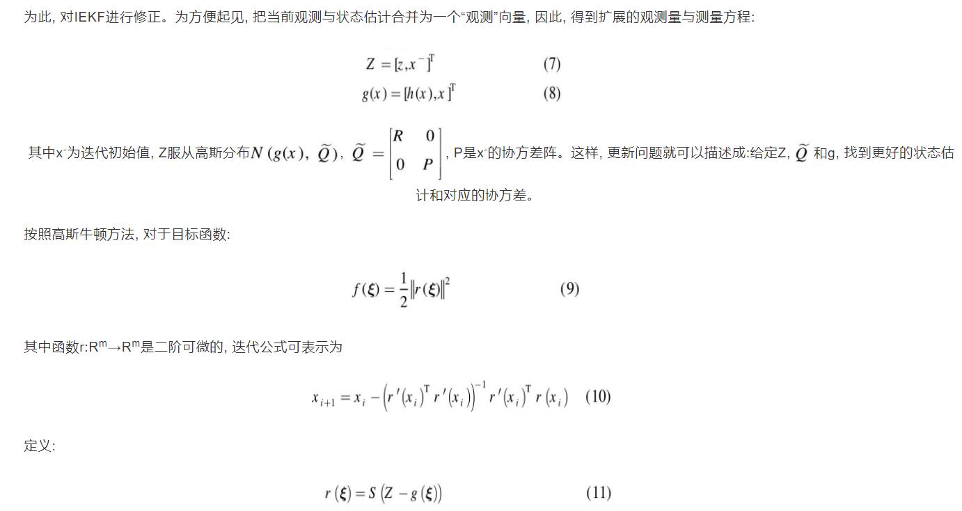
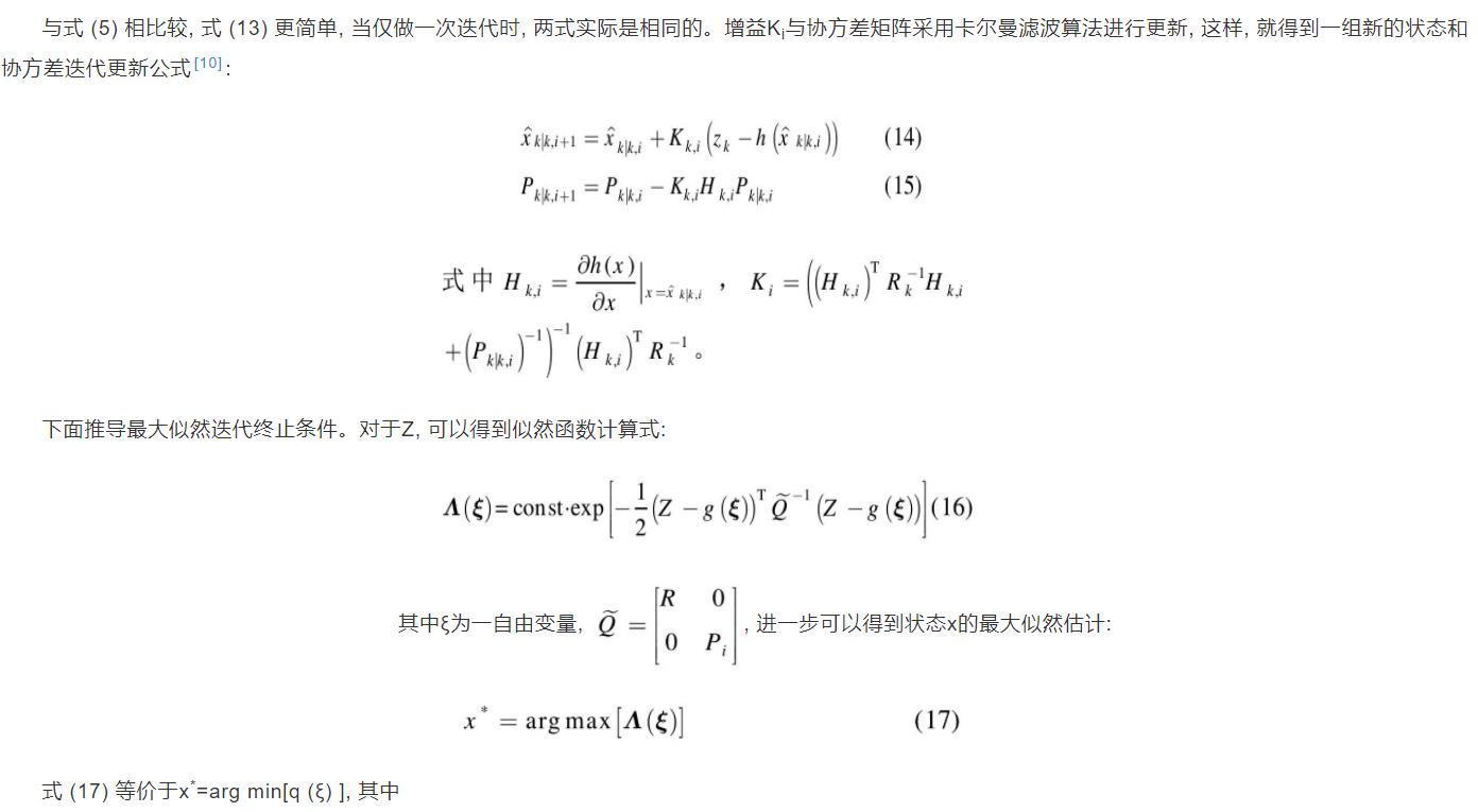
为此, 对IEKF进行修正。为方便起见, 把当前观测与状态估计合并为一个“观测”向量, 因此, 得到扩展的观测量与测量方程:

三、部分源代码

% function to implement the Iterated Extended Kalman Filter (IEKF)
% Inputs:
%  OBSn - the observations (with noise)
%  xest - initial state space estimates
% Ouputs:
%  Xp - predicted states
function Xp = f_IEKF(OBSn,xest)

load avar % r1,r2, L, and T

tol = .1; % tolerance for iterations
diff = 1;
count = 0;

F = [1 T 0 0 0 0 0;
    0 1 0 0 0 0 0;
    0 0 1 T 0 0 0;
    0 0 0 1 0 0 0;
    0 0 0 0 1 0 T;
    0 0 0 0 0 1 T;
    0 0 0 0 0 0 1]; % state transition matrix

n = size(OBSn,2); % number of observations

Xp = zeros(7,n);  % make room

Pkp1 = 1e10*eye(7); %xest*xest'; %.1*ones(7,7);

%Pkp1 = xest*xest';
%Pkp1 = F*Pkp1*F';

%Pkp1 = (10*randn(7,1))*(10*randn(7,1)).';
%Pkp1 = F*Pkp1*F';

% for each observation
for i = 1:n;
    
    % if this is the first iteration the prior predicted estimate is xest
    % if this is not the first run the prior estimate is in Xp
    if i == 1
        xkm1 = xest;
    else
        xkm1 = Xp(:,i-1);
    end
    
    Pkm1 = Pkp1; % conditional covariance from last iteration
    
    % iterations are started with the predicted estimate from the last run
    xkn = xkm1;
    while ~(diff < tol || count > 9)
        
        count = count + 1; 
        
        H = [gradest(@(x)f_h1(x),xkn); gradest(@(x)f_h2(x),xkn)];
        
        R = (.01*randn(2,1))*(.01*randn(2,1)).';
        
        Rdiag = diag(R); R = diag(Rdiag);
        
        K = Pkm1*H'*(H*Pkm1*H'+R)^-1;
        
        xkn_temp = xkm1 + K*(OBSn(:,i)-f_h(xkn)-H*(xkm1-xkn));
        
        diff = norm(abs(xkn_temp-xkn));
        
        fprintf('diff = %g \\n',diff)
        
        xkn = xkn_temp;
            
    end
    
    H = [gradest(@(x)f_h1(x),xkn); gradest(@(x)f_h2(x),xkn)];
    
    Pkk = (eye(7)-K*H)*Pkm1;
    
    Pkp1 = F*Pkk*F';
    
    Xp(:,i) = F*xkn;
    
    clc;
    
    fprintf('i = %g; Count is %g \\n',i,count)
    
    count = 0;
    
    diff = 1;
    
end

 
 % Script to start playing around with this stuff
clc; clear all; close all

% x  = [xc xcd zc zcd p1 p2 w].'

% simulation parameters
n = 100;                             % number of frames
xint = [-35 .7 35 .4 1 3 1].';       % initial state variable 
xest = [-32 .9 32 .6 1.2 2.2 .7].';  % initial state estimates
noise = .01;

% simulate dynamics
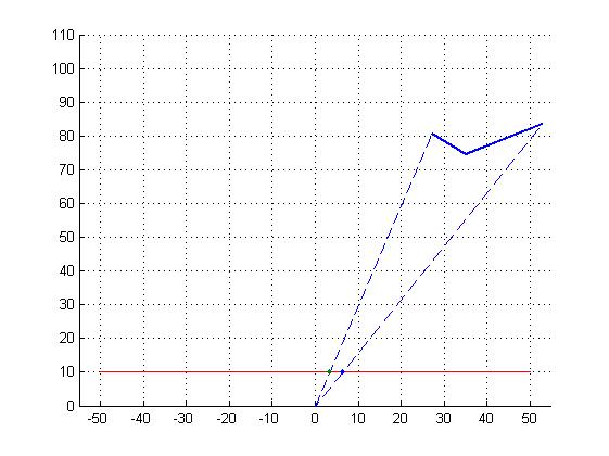
X = f_Simulate(xint,n);

% simulate observations
[OBS, OBSn] = f_Observe(X,noise);

% make movie
f_Movie(X,OBS,'SimMovie')

% run filter 
Xp = f_IEKF(OBSn,xest);

% make movie
OBSr = f_Observe(Xp,0);
f_Movie(Xp,OBSr,'ResultsMovie')

save RunData 

% pixel values
figure; 
pos = get(gcf,'Position');
set(gcf,'Position',[pos(1)-100 pos(2)-200 1.5*pos(3) 1.5*pos(4)]);
plot(1:n,OBSn,'.-',1:n,OBSr,'.-'); grid on;
legend('X1 simulated','X2 simulated','X1 predicted','X2 predicted','Location','Best')
xlabel('Frame index (n)','FontName','Time','FontSize',15); 
ylabel('Image pixel value','FontName','Time','FontSize',15); 
title('Pixel observations with noise',...
    'FontName','Time','FontSize',15,'FontWeight','Bold'); 

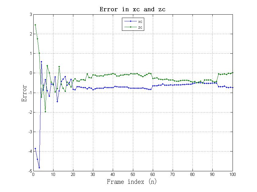
Error = X - Xp;
 
% error (xc and zc)
figure; 
pos = get(gcf,'Position');
set(gcf,'Position',[pos(1)-100 pos(2)-200 1.5*pos(3) 1.5*pos(4)]);
plot(1:n,Error([1 3],:),'.-'); grid on;
legend('xc','zc','Location','Best')
xlabel('Frame index (n)','FontName','Time','FontSize',15); 
ylabel('Error','FontName','Time','FontSize',15); 
title('Error in xc and zc',...
    'FontName','Time','FontSize',15,'FontWeight','Bold'); 

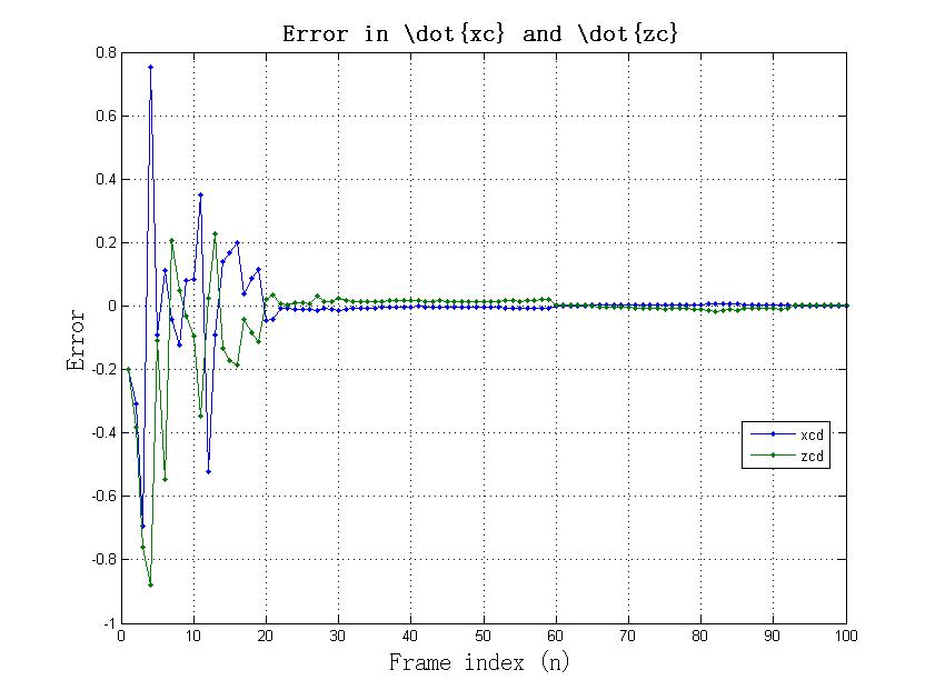
% error (xcd and zcd)
figure; 
pos = get(gcf,'Position');
set(gcf,'Position',[pos(1)-100 pos(2)-200 1.5*pos(3) 1.5*pos(4)]);
plot(1:n,Error([2 4],:),'.-'); grid on;
legend('xcd','zcd','Location','Best')
xlabel('Frame index (n)','FontName','Time','FontSize',15); 
ylabel('Error','FontName','Time','FontSize',15); 
title('Error in \\dotxc and \\dotzc',...
    'FontName','Time','FontSize',15,'FontWeight','Bold'); 

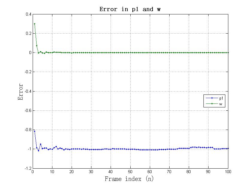
% error (p1 w)
figure; 
pos = get(gcf,'Position');
set(gcf,'Position',[pos(1)-100 pos(2)-200 1.5*pos(3) 1.5*pos(4)]);
plot(1:n,Error([5 7],:),'.-'); grid on;
legend('p1','w','Location','Best')
xlabel('Frame index (n)','FontName','Time','FontSize',15); 
ylabel('Error','FontName','Time','FontSize',15); 
title('Error in p1 and w',...
    'FontName','Time','FontSize',15,'FontWeight','Bold'); 

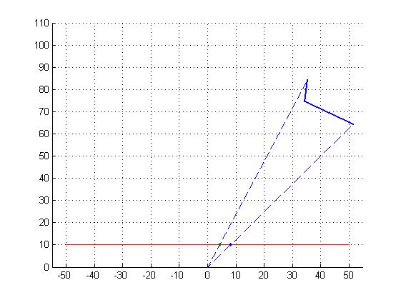
四、运行结果

五、matlab版本及参考文献

1 matlab版本
2014a

2 参考文献
[1] 包子阳,余继周,杨杉.智能优化算法及其MATLAB实例（第2版）[M].电子工业出版社，2016.
[2]张岩,吴水根.MATLAB优化算法源代码[M].清华大学出版社，2017.
[3]张俊根,姬红兵.IMM迭代扩展卡尔曼粒子滤波跟踪算法[J].电子与信息学报. 2010,32(05)