元胞自动机基于matlab元胞自动机HIV扩散模拟含Matlab源码 1292期

Posted 2021-09-20 紫极神光

一、元胞自动机简介

1 元胞自动机发展历程
最初的元胞自动机是由冯 · 诺依曼在 1950 年代为模拟生物 细胞的自我复制而提出的. 但是并未受到学术界重视.
1970 年, 剑桥大学的约翰 · 何顿 · 康威设计了一个电脑游戏 “生命游戏” 后, 元胞自动机才吸引了科学家们的注意.

1983 年 S.Wolfram 发表了一系列论文. 对初等元胞机 256 种 规则所产生的模型进行了深入研究, 并用熵来描述其演化行 为, 将细胞自动机分为平稳型, 周期型, 混沌型和复杂型.

2 对元胞自动机的初步认识
元胞自动机（CA）是一种用来仿真局部规则和局部联系的方法。典型的元胞自动机是定义在网格上的，每一个点上的网格代表一个元胞与一种有限的状态。变化规则适用于每一个元胞并且同时进行。典型的变化规则，决定于元胞的状态，以及其（ 4 或 8 ）邻居的状态。

3 元胞的变化规则&元胞状态
典型的变化规则，决定于元胞的状态，以及其（ 4 或 8 ）邻居的状态。

4 元胞自动机的应用
元胞自动机已被应用于物理模拟，生物模拟等领域。

5 元胞自动机的matlab编程
结合以上，我们可以理解元胞自动机仿真需要理解三点。一是元胞，在matlab中可以理解为矩阵中的一点或多点组成的方形块，一般我们用矩阵中的一点代表一个元胞。二是变化规则，元胞的变化规则决定元胞下一刻的状态。三是元胞的状态，元胞的状态是自定义的，通常是对立的状态，比如生物的存活状态或死亡状态，红灯或绿灯，该点有障碍物或者没有障碍物等等。

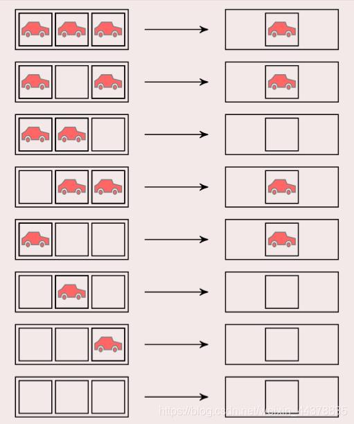
6 一维元胞自动机——交通规则
定义：
6.1 元胞分布于一维线性网格上.
6.2 元胞仅具有车和空两种状态.

7 二维元胞自动机——生命游戏
定义：
7.1 元胞分布于二维方型网格上.
7.2 元胞仅具有生和死两种状态.

元胞状态由周围八邻居决定.
规则：

骷髅：死亡；笑脸：生存
周围有三个笑脸，则中间变为笑脸
少于两个笑脸或者多于三个，中间则变死亡。

8 什么是元胞自动机
离散的系统: 元胞是定义在有限的时间和空间上的, 并且元 胞的状态是有限.
动力学系统: 元胞自动机的举止行为具有动力学特征.
简单与复杂: 元胞自动机用简单规则控制相互作用的元胞 模拟复杂世界.

9 构成要素

（1）元胞 (Cell)

元胞是元胞自动机基本单元：
状态: 每一个元胞都有记忆贮存状态的功能.
离散: 简单情况下, 元胞只有两种可能状态; 较复杂情况下, 元胞具有多种状态.
更新: 元胞的状态都安照动力规则不断更新.
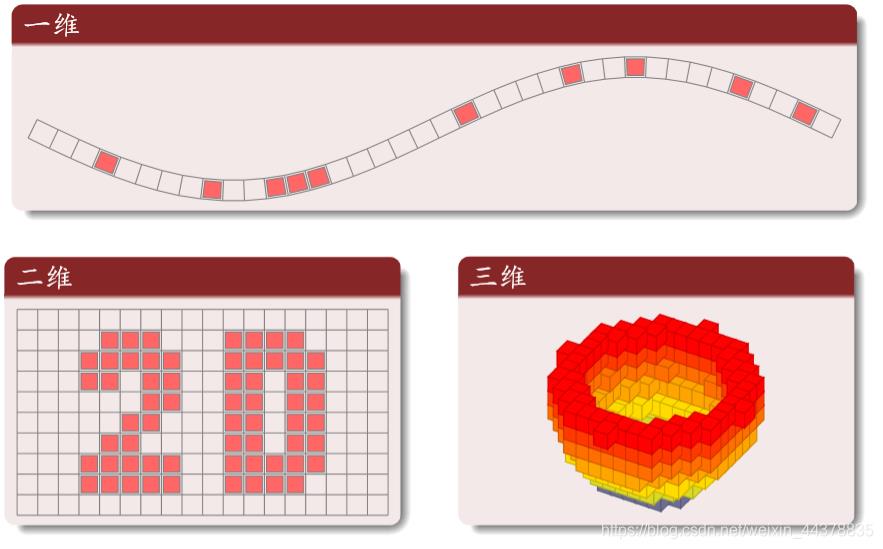
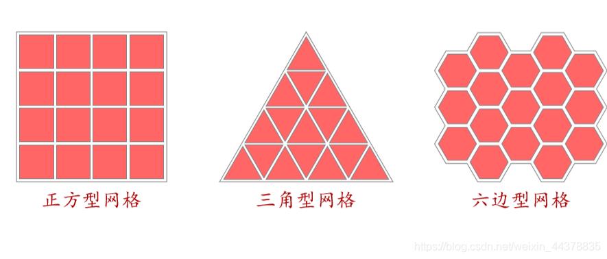
（2）网格 (Lattice)
不同维网格

常用二维网格

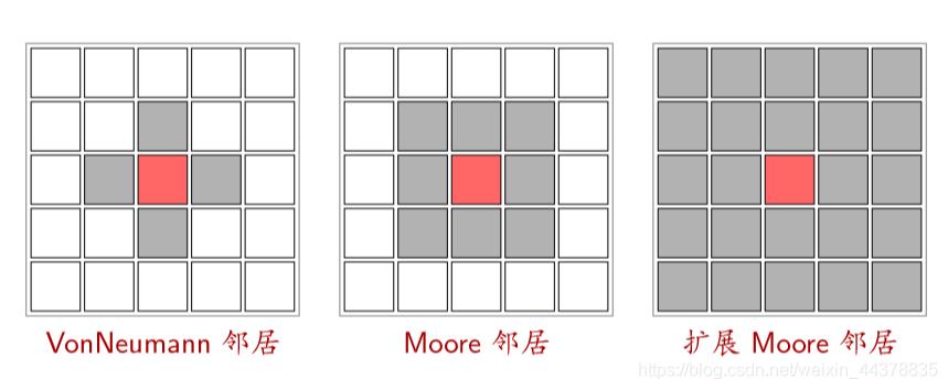
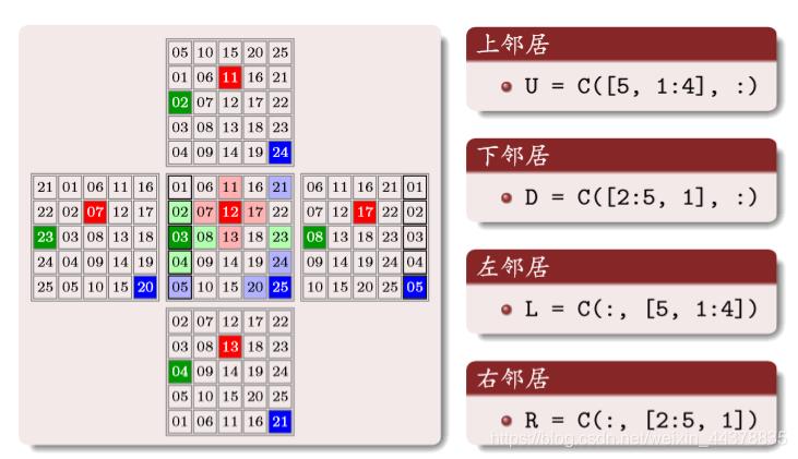
（3）邻居 (Neighborhood)

（4）边界 (Boundary)

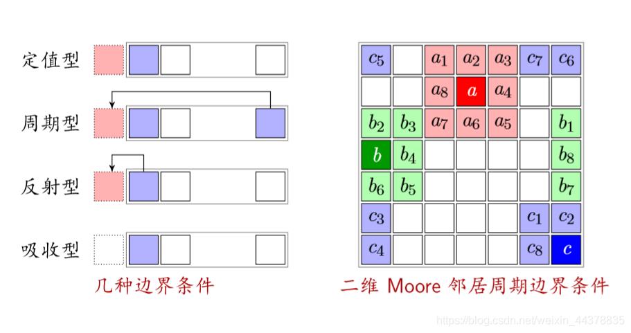
反射型：以自己作为边界的状态
吸收型：不管边界（车开到边界就消失）

（5）规则（状态转移函数）
定义：根据元胞当前状态及其邻居状况确定下一时刻该元胞状态的动力学函数, 简单讲, 就是一个状态转移函数.
分类 ：
总和型: 某元胞下时刻的状态取决于且仅取决于它所有邻居 的当前状态以及自身的当前状态.
合法型: 总和型规则属于合法型规则. 但如果把元胞自动机 的规则限制为总和型, 会使元胞自动机具有局限性.
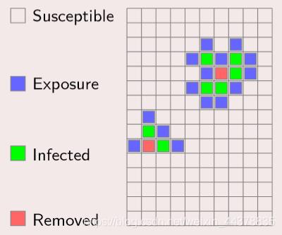
（6）森林火灾

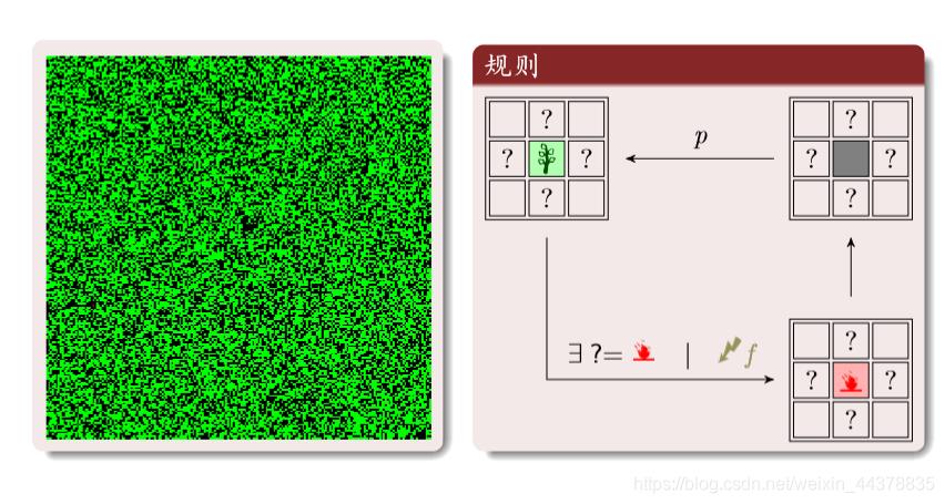
绿色：树木；红色：火；黑色：空地。
三种状态循环转化：
树：周围有火或者被闪电击中就变成火。
空地：以概率p变为树木
理性分析：红为火；灰为空地；绿是树

元胞三种状态的密度和为1

火转化为空地的密度等于空地转换为树的密度（新长出来的树等于烧没的树）

f是闪电的概率:远远小于树生成的概率；T s m a x T_{smax}T smax
​是一大群树被火烧的时间尺度
程序实现
周期性边界条件
购进啊

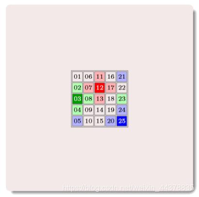
其中的数字为编号
构建邻居矩阵

上面矩阵中的数字编号，对应原矩阵相同位置编号的上邻居编号，一 一对应
同样道理：

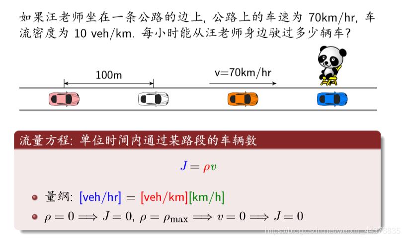
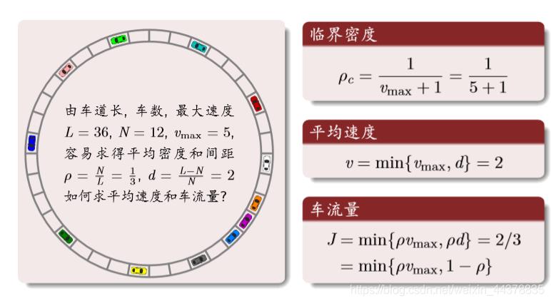
（7）交通概念
车距和密度

流量方程

守恒方程

时空轨迹（横轴是空间纵轴为时间）

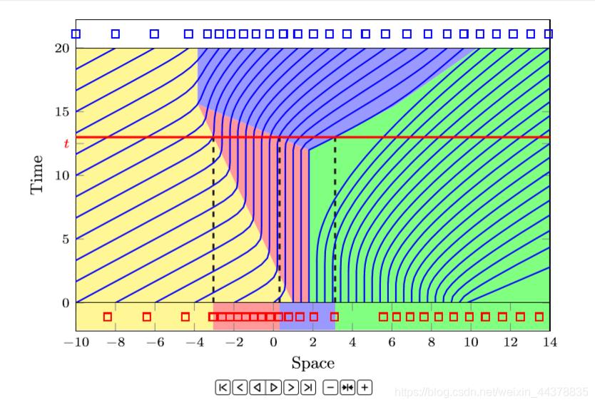
红线横线与蓝色交点表示每个时间车的位置。
如果是竖线则表示车子在该位置对应的时间

宏观连续模型：

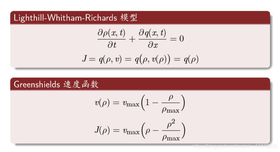
最常用的规则：

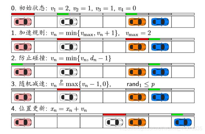
红色条表示速度是满的。

1 加速规则：不能超过v m a x （ 2 格 / s ） v_{max}（2格/s）v
max（2格/s）
2 防止碰撞：不能超过车距

理论分析：

结果分析: 密度与流量

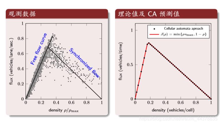
第一个图：横坐标是归一化后的密度，纵坐标是车流量。第二个图：理论值与CA的结果

结果分析: 时空轨迹

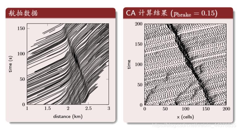
中间的深色区域是交通堵塞的区域。

二、部分源代码

     %% NOTE

% Total runtime for this code was about 1-3 minutes on the personal 
% computer used by the original researcher
% This runtime is expected to vary from device to device, and is being used 
% here to obtain a general comparison for runtime for the different
% models. It is not for a universal runtime value

%% Documentation

% n             size of each dimension of our square cellular automata grid
% P_HIV         fraction (probability) of cells initially infected by virus
% P_i           probability of a healthy cell becoming infected if its
%               neighborhood contains 1 I1 cell or X I2 cells
% P_v           probability of a healthy cell becoming infected by coming
%               in contact with a virus randomly (not from its
%               neighborhood)
% P_rep          Probability of a dead cell becoming replaced by a healthy
%               cell
% P_repI          Probability of a dead cell becoming replaced by an infected
%               cell
% X             Number of I2 cells in the neighborhood of an H cell that
%               can cause it to become infected
% tau1          tau1 is the number of timesteps it takes for an acute
%               infected cell to become latent.
% tau2          tau2 is the number of timesteps it takes for a latent
%               infected cell to become dead.
% totalsteps    totalsteps is the total number of steps of the CA (the
%               total number of weeks of simulations)
% grid          our cellular automata (CA) grid
% tempgrid      tempgrid is a temporary grid full of random numbers that is
%               used to randomly add different states to our CA grid.
% taugrid       taugrid is a grid the same size as our CA grid that stores
%               the number of timesteps that a cell has been in state I_1.
%               If the number reaches tau1, then the state changes to I_2.
% state         state is a [5 x totalsteps] size matrix that stores
%               the total number of cells in each state at each timestep
%               and the last row stores sum of I_1 and I_2 at each timestep
% timestep      each simulation step of the cellular automata
%               1 timestep = 1 week of time in the real world
% nextgrid      nextgrid is a temporary grid. It is a copy of the CA grid
%               from the previous simulation. It stores all the CA rule
%               updates of the current timestep and stores it all back to
%               the grid to display.

%% Clean-up

clc;            % clears command window
clear all;      % clears workspace and deletes all variables
close all;      % closes all open figures

%% Parameters

n = 100;            % meaning that our grid will have the dimensions n x n
P_HIV = 0.05;      % initial grid will have P_hiv acute infected cells
P_i = 0.997;        % probability of infection by neighbors
P_v = 0.00001;      % probability of infection by random viral contact
P_rep = 0.99;        % probability of dead cell being replaced by healthy
P_repI = 0.00001;     % probability of dead cell being replaced by infected
X = 4;              % there must be at least X I_2 neighbors to infect cell
tau1 = 4;           % time delay for I_1 cell to become I_2 cell
tau2 = 1;           % time delay for I_2 cell to become D cell
totalsteps = 600 ;  % total number of weeks of simulation to be performed
savesteps = [3 7 11 15 20 25 50 100 150 200 250 300 350 400 450 500]; 
                    %timesteps for which we want to save simulation image

%% States

% State 1: H:   Healthy          (Color- Green)
% State 4: I_1: Active Infected  (Color- Cyan)
% State 3: I_2: Latent Infected  (Color- Blue)
% State 2: D:   Dead             (Color- Black)

%% Initial Grid


grid = ones(n);     % creates our initial n x n matrix and fills all cells
% with value 1 (meaning H state - Healthy cell)
tempgrid = rand(n); % creates a grid of random values of the same size as
% our CA grid. Used to randomly add I_1 state to our grid
grid(tempgrid(:,:)<=P_HIV) = 4;  % I_1 state added with probability  P_HIV

% The following sets the edge values of the grid to H state
grid(:,[1 n]) = 1;   % to set every value in the first and last column to 1
grid([1 n],:) = 1;   % to set every value in the first and last row to 1

% NOTE: Our CA only simulates from rows 2 to n-1, and columns 2 to n-1.
%       This is to prevent the edge row and column cells from having an
%       out-of-bounds error when checking the neighbors around them.
%       The edge values are all set to H state so that it does not affect
%       Rule 1 of the CA for cells next to them

% set(figure, 'OuterPosition', [100 30 740 740]) % sets figure window size
% % outerposition values are [left, bottom, width, height]
% print1(grid);   % prints the initial grid
% saveas(gcf,strcat('Model1Timestep0.pdf'));

%% Simulation

    nextgrid = grid;
    for x=2:n-1
        for y=2:n-1
            
            % Rule 1
            % If the cell is in H state and at least one of its neighbors
            % is in I_1 state, or X of its neighbors is in I_2 state, then
            % the cell becomes I_1 with a probability of P_i
            % The cell may also becomes I_1 by randomly coming in
            % contact with a virus from outside its neighborhood with a
            % probability of P_v
            if(grid(x,y)==1)
                if((rand<=P_i && (grid(x-1,y-1)==4 || grid(x-1,y)==4 || ...
                        grid(x-1,y+1)==4 || grid(x,y-1)==4 || ...
                        grid(x,y+1)==4 || grid(x+1,y-1)==4 || ...
                        grid(x+1,y)==4 || grid(x+1,y+1)==4 || ...
                        ((grid(x-1,y-1)==3) + (grid(x-1,y)==3) + ...
                        (grid(x-1,y+1)==3) + (grid(x,y-1)==3) + ...
                        (grid(x,y+1)==3) + (grid(x+1,y-1)==3) + ...
                        (grid(x+1,y)==3) + (grid(x+1,y+1)==3))>=X ))...
                        || rand<=P_v)                    
 
                end
     
            end
            
            % Rule 2
            % If the cell is in state I_1, and has been in this state for
            % tau1 timesteps, the cell becomes I_2 state (latent infected)
            if((grid(x,y)==4))
                taugrid(x,y) = taugrid(x,y)+1;
                if(taugrid(x,y)==tau1)
                    nextgrid(x,y)=3;
                    taugrid(x,y)=0;
                end
                continue;
            end
            
            % Rule 3
            % If the cell is in I_2 state, and has been in this state for
            % tau2 timesteps, the cell becomes D state (dead)
            % Since tau2=1, this rule is implemented every timestep
            if((grid(x,y)==3))
                nextgrid(x,y)=2;
                continue;
            end
            
            % Rule 4 a and b
            % If the cell is in D state, then the cell will become H state
            % with probability P_rep (4.a) or I_1 state with probability
            % P_repI (4.b)
            if(grid(x,y)==2 && rand<=P_rep)
                if(rand<=P_repI)
                    nextgrid(x,y)=4;
                    continue;
                else
                    nextgrid(x,y)=1;
                end
            end
            
        end
    end
    % to assign the updates of this timestep in nextgrid back to our grid
    grid=nextgrid;          
    % to display the grid at the end of each timestep
    print1(grid);
    % to save the image of the simulation every 25 timesteps as a pdf
    if(find(savesteps==timestep))
        saveas(gcf,strcat('Model1Timestep',num2str(timestep),'.pdf'));
    end
    
    state(1,timestep) = sum(sum(grid(2:n-1,2:n-1)==1));
    state(2,timestep) = sum(sum(grid(2:n-1,2:n-1)==2));
    state(3,timestep) = sum(sum(grid(2:n-1,2:n-1)==3));
    state(4,timestep) = sum(sum(grid(2:n-1,2:n-1)==4));
    
    timestep=timestep+1;    % to move to the next timestep
end

% The following lines of code are to display a graph of each state of
% cells during simulation
set(figure, 'OuterPosition', [200 100 700 500]) % sets figure window size
plot( 1:totalsteps , state(1,:), 'g', ...
    1:totalsteps , state(4,:), 'c', ...
    1:totalsteps , state(3,:), 'b', ...
    1:totalsteps , state(2,:), 'k' , 'linewidth', 2 );
legend( 'Healthy', 'Acute Infected', 'Latent Infected', 'Dead', ...
    'Location' ,'NorthEast' );
saveas(gcf,strcat('Model1GraphSingleRun.pdf'));
error(nargchk(1,Inf,nargin)) ;

% check the arguments
if ~isnumeric(x),
    error('Numeric argument expected') ;
end

if nargin==1,
    y = [] ;
    va = [] ;
else
    va = varargin ;
    if ischar(va{1}),
        % optional arguments are
        y = [] ;
    elseif isnumeric(va{1})        
        y = va{1} ;
        va = va(2:end) ;
    else
        error('Invalid second argument') ;
    end
    if mod(size(va),2) == 1,
        error('Property-Value have to be pairs') ;
    end
end

% get the axes to plot in
hca=get(get(0,'currentfigure'),'currentaxes');
if isempty(hca),
    warning('No current axes found') ;
    return ;
end

% get the current limits of the axis
% used for limit restoration later on
xlim = get(hca,'xlim') ;
ylim = get(hca,'ylim') ;

% setup data for the vertical lines
xx1 = repmat(x(:).',3,1) ;
yy1 = repmat([ylim(:) ; nan],1,numel(x)) ;

三、运行结果

四、matlab版本及参考文献

1 matlab版本
2014a

2 参考文献
[1] 蔡利梅.MATLAB图像处理——理论、算法与实例分析[M].清华大学出版社，2020.
[2]杨丹,赵海滨,龙哲.MATLAB图像处理实例详解[M].清华大学出版社，2013.
[3]周品.MATLAB图像处理与图形用户界面设计[M].清华大学出版社，2013.
[4]刘成龙.精通MATLAB图像处理[M].清华大学出版社，2015.
[5]孟逸凡,柳益君.基于PCA-SVM的人脸识别方法研究[J].科技视界. 2021,(07)
[6]张娜,刘坤,韩美林,陈晨.一种基于PCA和LDA融合的人脸识别算法研究[J].电子测量技术. 2020,43(13)
[7]陈艳.基于BP神经网络的人脸识别方法分析[J].信息与电脑(理论版). 2020,32(23)
[8]戴骊融,陈万米,郭盛.基于肤色模型和SURF算法的人脸识别研究[J].工业控制计算机. 2014,27(02)