小白学习PyTorch教程十三迁移学习：微调Alexnet实现ant和bee图像分类

Posted 2021-08-28 刘润森！

tags:

篇首语：本文由小常识网(cha138.com)小编为大家整理，主要介绍了小白学习PyTorch教程十三迁移学习：微调Alexnet实现ant和bee图像分类相关的知识，希望对你有一定的参考价值。

@Author：Runsen

上次微调了VGG19，这次微调Alexnet实现ant和bee图像分类。

多年来，CNN许多变体已经发展起来，从而产生了几种 CNN 架构。其中最常见的是：

LeNet-5 (1998)
AlexNet (2012)
ZFNet (2013)
GoogleNet / Inception（2014）
VGGNet (2014)
ResNet (2015)

这篇博客是关于AlexNet 教程，AlexNet 也是之前受欢迎的 CNN 架构之一。

AlexNet

AlexNet主要由 Alex Krizhevsky 设计。它由 Ilya Sutskever 和 Krizhevsky 的博士生导师 Geoffrey Hinton 共同发表，是卷积神经网络或 CNN。

在参加 ImageNet 大规模视觉识别挑战赛后，AlexNet 一举成名。Alexnet在分类任务中实现了 84.6% 的前 5 名准确率，而排名第二的团队的前 5 名准确率为 73.8%。由于 2012 年的计算能力非常有限，Alex 在 2 个 GPU 上对其进行了训练。

上图是2012 Imagenet 挑战赛的 Alexnet 架构

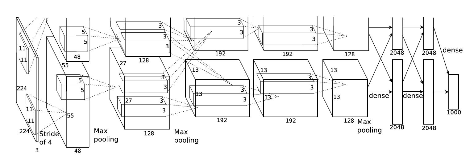
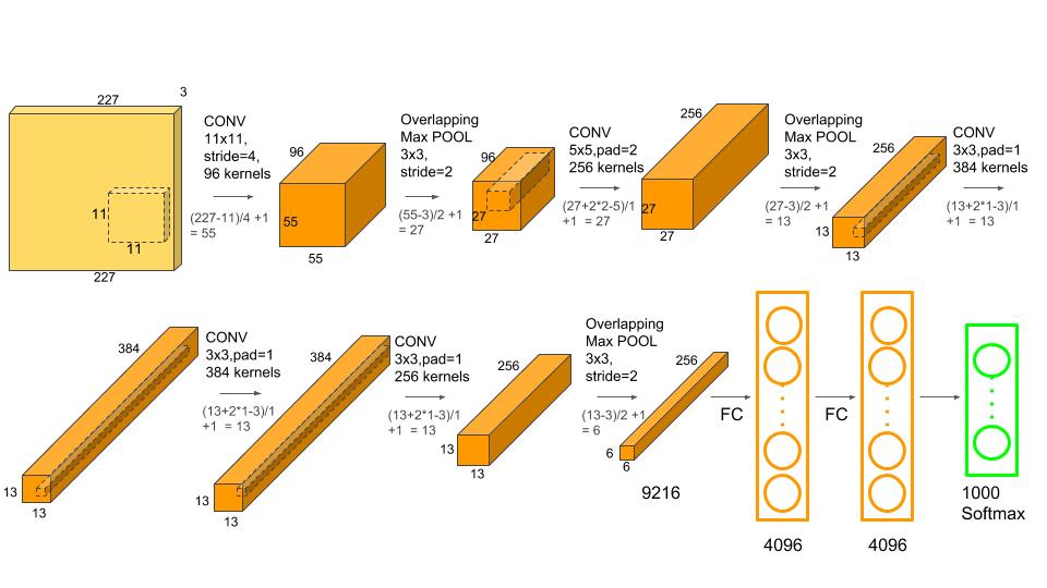
AlexNet 架构由 5 个卷积层、3 个最大池化层、2 个归一化层、2 个全连接层和 1 个 softmax 层组成。
每个卷积层由卷积滤波器和非线性激活函数ReLU组成。
池化层用于执行最大池化。
由于全连接层的存在，输入大小是固定的。
输入大小之前在大多数被提及为 224x224x3，但由于一些填充，变成了 227x227x3
AlexNet 总共有 6000 万个参数。

下面是Alexnet中的 227x227x3 模型参数

Size / Operation	Filter	Depth	Stride	Padding	Number of Parameters	Forward Computation
3* 227 * 227
Conv1 + Relu	11 * 11	96	4		(11 * 11 3 + 1) 96=34944	(11113 + 1) * 96 * 55 * 55=105705600
96 * 55 * 55
Max Pooling	3 * 3		2
96 * 27 * 27
Norm
Conv2 + Relu	5 * 5	256	1	2	(5 * 5 * 96 + 1) * 256=614656	(5 * 5 * 96 + 1) * 256 * 27 * 27=448084224
256 * 27 * 27
Max Pooling	3 * 3		2
256 * 13 * 13
Norm
Conv3 + Relu	3 * 3	384	1	1	(3 * 3 * 256 + 1) * 384=885120	(3 * 3 * 256 + 1) * 384 * 13 * 13=149585280
384 * 13 * 13
Conv4 + Relu	3 * 3	384	1	1	(3 * 3 * 384 + 1) * 384=1327488	(3 * 3 * 384 + 1) * 384 * 13 * 13=224345472
384 * 13 * 13
Conv5 + Relu	3 * 3	256	1	1	(3 * 3 * 384 + 1) * 256=884992	(3 * 3 * 384 + 1) * 256 * 13 * 13=149563648
256 * 13 * 13
Max Pooling	3 * 3		2
256 * 6 * 6
Dropout (rate 0.5)
FC6 + Relu					256 * 6 * 6 * 4096=37748736	256 * 6 * 6 * 4096=37748736
4096
Dropout (rate 0.5)
FC7 + Relu					4096 * 4096=16777216	4096 * 4096=16777216
4096
FC8 + Relu					4096 * 1000=4096000	4096 * 1000=4096000
1000 classes
Overall					62369152=62.3 million	1135906176=1.1 billion
Conv VS FC					Conv:3.7million (6%) , FC: 58.6 million (94% )	Conv: 1.08 billion (95%) , FC: 58.6 million (5%)

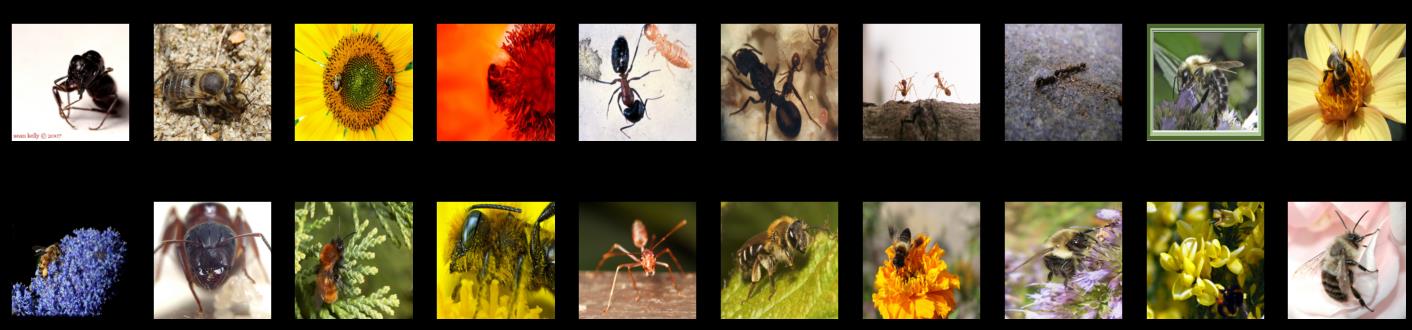
数据集介绍

本数据集中存在PyTorch相关入门的数据集ant和bee案例，每一个ant和bee

数据来源：PyTorch深度学习快速入门教程（绝对通俗易懂！）【小土堆】

关于数据集和代码见文末

读取数据

这里选择将数据reshape成224*224。

import torch
import numpy as np
import matplotlib.pyplot as plt
import torch.nn.functional as F
from torch import nn
from torchvision import datasets, transforms, models

device = torch.device('cuda:0' if torch.cuda.is_available() else "cpu")

#transforms
transform_train = transforms.Compose([transforms.Resize((224, 224)),
                                      transforms.RandomHorizontalFlip(),
                                      transforms.RandomAffine(0, shear=10, scale=(0.8, 1.2)),
                                      transforms.ColorJitter(brightness=1, contrast=1, saturation=1),
                                      transforms.ToTensor(),
                                      transforms.Normalize((0.5, 0.5, 0.5), (0.5, 0.5, 0.5))
                                    ])

transform = transforms.Compose([transforms.Resize((224, 224)),
                               transforms.ToTensor(),
                               transforms.Normalize((0.5, 0.5, 0.5), (0.5, 0.5, 0.5))
                               ])
root_train = 'ants_and_bees/train'
root_val = 'ants_and_bees/val'

training_dataset = datasets.ImageFolder(root=root_train, transform=transform)
validation_dataset = datasets.ImageFolder(root=root_val, transform=transform)
training_loader = torch.utils.data.DataLoader(training_dataset, batch_size=20, shuffle=True)
validation_loader = torch.utils.data.DataLoader(validation_dataset, batch_size = 20, shuffle=False)

展示数据

dataiter = iter(training_loader)
images, labels = dataiter.next()
fig = plt.figure(figsize=(25,6))

def im_convert(tensor):
  image = tensor.cpu().clone().detach().numpy()
  image = image.transpose(1, 2, 0) #shape 32 x 32 x 1
  #de-normalisation - multiply by std and add mean
  image = image * np.array((0.5, 0.5, 0.5)) + np.array((0.5, 0.5, 0.5))
  image = image.clip(0, 1)
  return image

for idx in np.arange(20):
  ax = fig.add_subplot(2, 10, idx+1, xticks=[], yticks=[])
  plt.imshow(im_convert(images[idx]))
  #print(labels[idx].item())
  ax.set_title(classes[labels[idx].item()])
plt.show()

微调Alexnet

model = models.alexnet(pretrained=True)
print(model)

AlexNet(
  (features): Sequential(
    (0): Conv2d(3, 64, kernel_size=(11, 11), stride=(4, 4), padding=(2, 2))
    (1): ReLU(inplace=True)
    (2): MaxPool2d(kernel_size=3, stride=2, padding=0, dilation=1, ceil_mode=False)
    (3): Conv2d(64, 192, kernel_size=(5, 5), stride=(1, 1), padding=(2, 2))
    (4): ReLU(inplace=True)
    (5): MaxPool2d(kernel_size=3, stride=2, padding=0, dilation=1, ceil_mode=False)
    (6): Conv2d(192, 384, kernel_size=(3, 3), stride=(1, 1), padding=(1, 1))
    (7): ReLU(inplace=True)
    (8): Conv2d(384, 256, kernel_size=(3, 3), stride=(1, 1), padding=(1, 1))
    (9): ReLU(inplace=True)
    (10): Conv2d(256, 256, kernel_size=(3, 3), stride=(1, 1), padding=(1, 1))
    (11): ReLU(inplace=True)
    (12): MaxPool2d(kernel_size=3, stride=2, padding=0, dilation=1, ceil_mode=False)
  )
  (avgpool): AdaptiveAvgPool2d(output_size=(6, 6))
  (classifier): Sequential(
    (0): Dropout(p=0.5, inplace=False)
    (1): Linear(in_features=9216, out_features=4096, bias=True)
    (2): ReLU(inplace=True)
    (3): Dropout(p=0.5, inplace=False)
    (4): Linear(in_features=4096, out_features=4096, bias=True)
    (5): ReLU(inplace=True)
    (6): Linear(in_features=4096, out_features=1000, bias=True)
  )
)

通过转移学习，我们将使用从卷积层中提取的特征
需要把最后一层的out_features=1000，改为out_features=2

因为我们的模型只对蚂蚁和蜜蜂进行分类，所以输出应该是2，而不是AlexNet的输出层中指定的1000。因此，我们改变了AlexNet中的classifier第6个元素的输出。

for param in model.features.parameters():
  `param.requires_grad = False                     

import torch.nn as nn

n_inputs = model.classifier[6].in_features      #4096
last_layer = nn.Linear(n_inputs, len(classes))
model.classifier[6] = last_layer
model.to(device)

print(model)

AlexNet(
  (features): Sequential(
    (0): Conv2d(3, 64, kernel_size=(11, 11), stride=(4, 4), padding=(2, 2))
    (1): ReLU(inplace=True)
    (2): MaxPool2d(kernel_size=3, stride=2, padding=0, dilation=1, ceil_mode=False)
    (3): Conv2d(64, 192, kernel_size=(5, 5), stride=(1, 1), padding=(2, 2))
    (4): ReLU(inplace=True)
    (5): MaxPool2d(kernel_size=3, stride=2, padding=0, dilation=1, ceil_mode=False)
    (6): Conv2d(192, 384, kernel_size=(3, 3), stride=(1, 1), padding=(1, 1))
    (7): ReLU(inplace=True)
    (8): Conv2d(384, 256, kernel_size=(3, 3), stride=(1, 1), padding=(1, 1))
    (9): ReLU(inplace=True)
    (10): Conv2d(256, 256, kernel_size=(3, 3), stride=(1, 1), padding=(1, 1))
    (11): ReLU(inplace=True)
    (12): MaxPool2d(kernel_size=3, stride=2, padding=0, dilation=1, ceil_mode=False)
  )
  (avgpool): AdaptiveAvgPool2d(output_size=(6, 6))
  (classifier): Sequential(
    (0): Dropout(p=0.5, inplace=False)
    (1): Linear(in_features=9216, out_features=4096, bias=True)
    (2): ReLU(inplace=True)
    (3): Dropout(p=0.5, inplace=False)
    (4): Linear(in_features=4096, out_features=4096, bias=True)
    (5): ReLU(inplace=True)
    (6): Linear(in_features=4096, out_features=2, bias=True)
  )
)

训练和测试模型

criterion = nn.CrossEntropyLoss()
optimizer = torch.optim.Adam(model.parameters(), lr=0.0001)

epochs = 5
losses = []
accuracy = []
val_losses = []
val_accuracies = []

for e in range(epochs):
  running_loss = 0.0
  running_accuracy = 0.0
  val_loss = 0.0
  val_accuracy = 0.0

  for images, labels in training_loader:
    images = images.to(device)
    labels = labels.to(device)
    outputs = model(images)   
    loss = criterion(outputs, labels)

    optimizer.zero_grad()
    loss.backward()
    optimizer.step()

    _, preds = torch.max(outputs, 1)
    running_accuracy += torch.sum(preds == labels.data)
    running_loss += loss.item() 

    #不必为验证集执行梯度
    with torch.no_grad():       
      for val_images, val_labels in validation_loader:
        val_images = val_images.to(device)
        val_labels = val_labels.to(device)
        val_outputs = model(val_images)
        val_loss = criterion(val_outputs, val_labels)

        _, val_preds = torch.max(val_outputs, 1)
        val_accuracy += torch.sum(val_preds == val_labels.data)
        val_loss += val_loss.item() 
    # metrics for training data
    epoch_loss = running_loss/len(training_loader.dataset)
    epoch_accuracy = running_accuracy.float()/len(training_loader.dataset)
    losses.append(epoch_loss)
    accuracy.append(epoch_accuracy)
    # metrics for validation data
    val_epoch_loss = val_loss/len(validation_loader.dataset)
    val_epoch_accuracy = val_accuracy.float()/len(validation_loader.dataset)
    val_losses.append(val_epoch_loss)
    val_accuracies.append(val_epoch_accuracy)
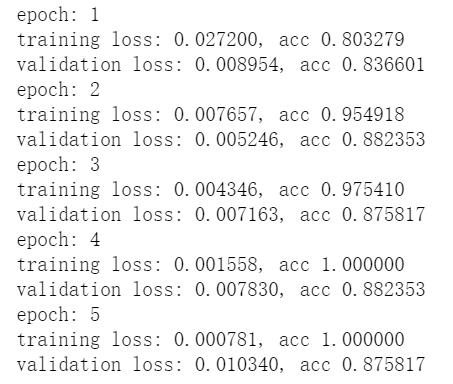
    #print the training and validation metrics
    print("epoch:", e+1)
    print('training loss: {:.6f}, acc {:.6f}'.format(epoch_loss, epoch_accuracy.item()))
    print('validation loss: {:.6f}, acc {:.6f}'.format(val_epoch_loss, val_epoch_accuracy.item()))

plt.plot(losses, label='training loss')
plt.plot(val_losses, label='validation loss&以上是关于小白学习PyTorch教程十三迁移学习：微调Alexnet实现ant和bee图像分类的主要内容，如果未能解决你的问题，请参考以下文章 
 小白学习PyTorch教程十二迁移学习：微调VGG19实现图像分类
 小白学习PyTorch教程十六在多标签分类任务上 微调BERT模型
 小白学习PyTorch教程十六在多标签分类任务上 微调BERT模型
 PyTorch迁移学习教程（计算机视觉应用实例)
 Pytorch Note56 Fine-tuning 通过微调进行迁移学习
 pytorch迁移学习