基于pandasmatplotlib和seaborn进行数据分析实战建议收藏
Posted 老吴^名字下个月说
tags:
篇首语:本文由小常识网(cha138.com)小编为大家整理,主要介绍了基于pandasmatplotlib和seaborn进行数据分析实战建议收藏相关的知识,希望对你有一定的参考价值。
项目来源:
https://www.kaggle.com/anthonypino/melbourne-housing-market
项目简介:
利用以往的房屋销售信息,分析哪种房屋最值得推荐给投资者进行投资。
PS: 本次项目是在jupyter上运行的。(文末附资源链接)
导入模块:
%matplotlib inline
import pandas as pd
import seaborn as sns
import statsmodels.formula.api as smf
from sklearn.linear_model import LinearRegression
from sklearn import metrics
from sklearn.model_selection  import train_test_split
import numpy as np
from scipy.stats import norm # for scientific Computing
from scipy import stats, integrate
import matplotlib.pyplot as plt
plt.rcParams['font.sans-serif'] = ['SimHei'] # 设置汉字字体,优先使用黑体
plt.rcParams['font.size'] = 12  # 设置字体大小
plt.rcParams['axes.unicode_minus'] = False   # 设置正常显示负号
加载数据:
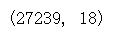
melbourne_data  = pd.read_csv("./Melbourne_housing_FULL.csv")
melbourne_data.head(10)

接下来正式开始进行分析啦!
1 数据探索与数据清洗
1.1 数据探索
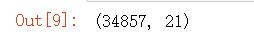
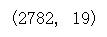
melbourne_data.shape
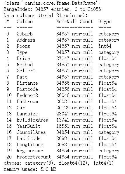
melbourne_data.info()

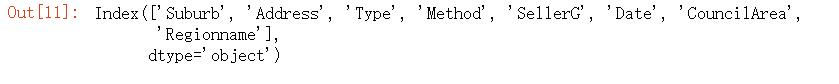
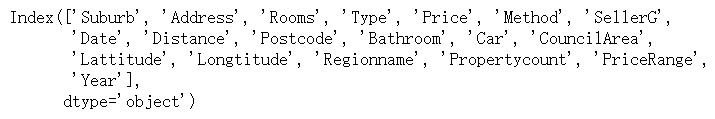
从上面的数据信息可以看出,非数值数据被视为对象。该列表包括以下列:“suburban”、“Address”、“Type”、“Method”、“SellerG”、“Date”、“councileArea”、“Regionname”。在接下来的几个步骤中,我们将把对象数据类型更改为category和Date数据类型。
# 验证字符串类型的数据
melbourne_data.select_dtypes(["object"]).columns
1.2 更换数据类型
# 将所有字符串数据类型更改为类别-此步骤对于能够绘制类别数据以进行分析是必需的
objdtype_cols = melbourne_data.select_dtypes(["object"]).columns
melbourne_data[objdtype_cols] = melbourne_data[objdtype_cols].astype('category')

melbourne_data.info()
## 看上面的数据信息,我们可以注意到“数据”也被转换成了类别。
## 在这一步中,我们将将日期转换为datetime
melbourne_data['Date'] =  pd.to_datetime( melbourne_data['Date'])

melbourne_data.info()

在接下来的几个步骤中,我们将对数值特征变量进行数据预处理。
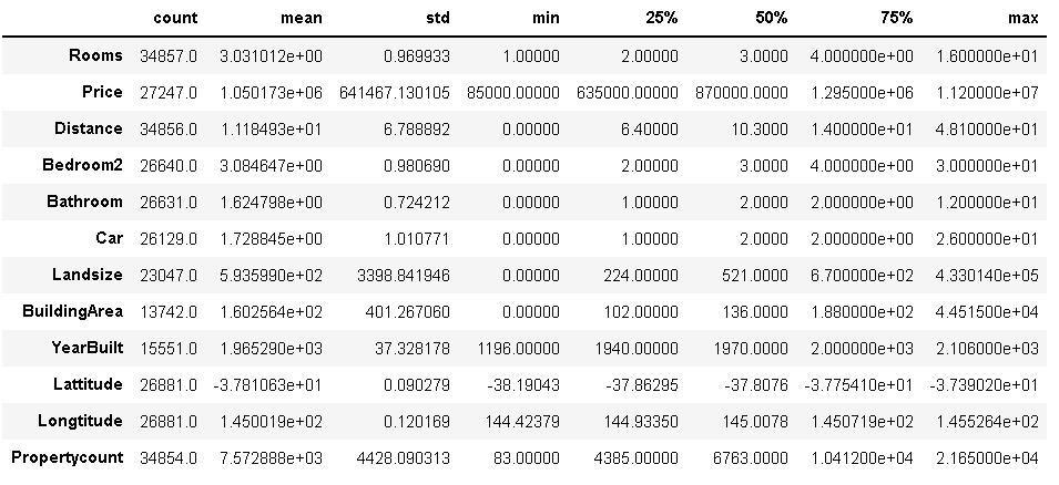
melbourne_data.describe().T
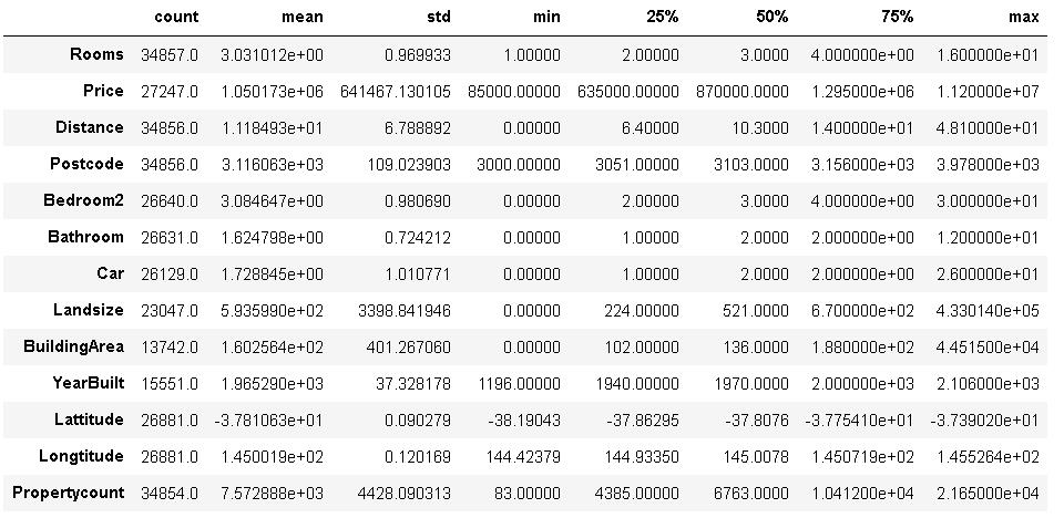
观察以上有关数字数据的信息,可以注意到邮政编码也被视为数字数据。既然我们知道邮政编码是一个分类数据,我们将把它分类。
melbourne_data["Postcode"] = melbourne_data["Postcode"].astype('category')

melbourne_data.describe().T
仔细评估数据后,可以注意到变量“Rooms”和“Bedroom2”非常相似,应该删除其中一列以避免重复数据。
## 在这一步中,我们将首先通过观察“Rooms”和“Bedroom2”来确认我们的上述声明
melbourne_data['b 2 r'] = melbourne_data["Bedroom2"] - melbourne_data["Rooms"]
melbourne_data[['b 2 r', 'Bedroom2', 'Rooms']].head()
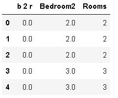
## 我们可以看到,这里的差别非常小,删除这两列中的一列是明智的
melbourne_data = melbourne_data.drop(['b 2 r', 'Bedroom2'], 1)
1.3 缺失值处理
我们可以使用多种方法来探索缺失的数据。在这里,我们将首先使用一个可视化的方式来获得一些提示。在后面的步骤中,我们将进行一些计算,以获得每个变量中丢失数据的确切数量。根据数据、我们的经验和业务需要,我们要么填写缺失的值,要么删除具有空值的行或列。
## 可视化缺失值
fig, ax = plt.subplots(figsize=(15,7))
sns.heatmap(melbourne_data.isnull(), yticklabels=False,cmap='viridis')
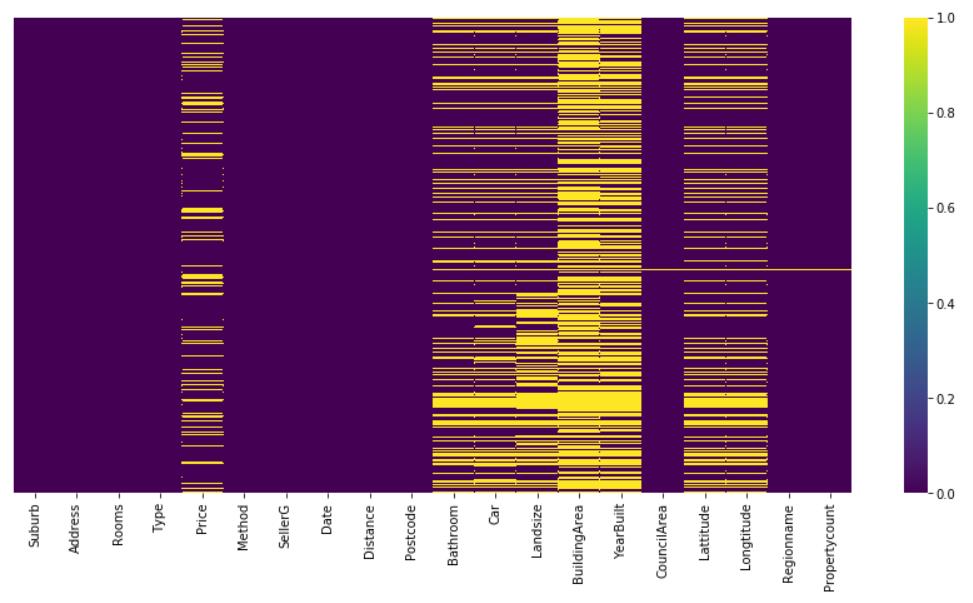
从上图可以得出结论,price,bathroom,car和landsize,lattitude和longtitude有部分缺失值,在buildingarea和bulityear中有许多缺少的值。在下一步中,让我们研究缺失值的计数。
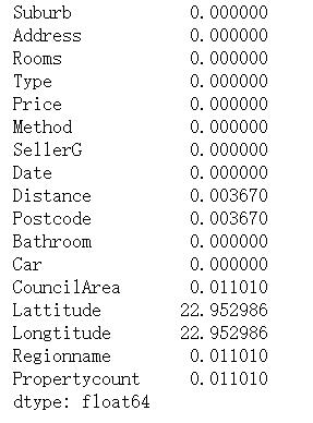
# 百分比缺失值
melbourne_data.isnull().sum()/len(melbourne_data)*100
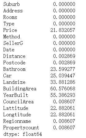
从上面的信息中,我们可以注意到很少的特性变量仍然有很大比例的缺失值。此时我们将忽略它,但在稍后的状态中,如果我们将这些作为后续的特征变量,我们将探索填充这些信息或从数据中删除这些信息的方法。
melbourne_data = melbourne_data.drop(["Landsize", "BuildingArea", "YearBuilt"], axis=1)
# 另外,因为我们的目标变量是price,所以在缺少price值时,删除price列的行是有意义的
melbourne_data.dropna(subset=["Price"], inplace=True)

melbourne_data['Car']=melbourne_data['Car'].fillna(melbourne_data['Car'].mode()[0])
melbourne_data['Bathroom']=melbourne_data['Bathroom'].fillna(melbourne_data['Bathroom'].mode()[0])

melbourne_data.shape

# 百分比缺失值
melbourne_data.isnull().sum()/len(melbourne_data)*100
1.4 寻找异常数据
异常值可以显著影响数据分析,也可以影响数据的规范化。在数据预处理过程中,识别和删除它们是非常重要的。在接下来的几个步骤中,我们将在数据中处理异常值(如果有的话)。
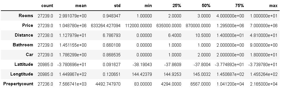
melbourne_data.describe().T

从上面的统计总结中我们可以看到,我们数据中的最高价格接近1120万美元。这看起来像是一个明显的异常值。但是在删除它之前,让我们首先确保在这个范围内只有很少的值。
# 为了找出异常值,我们将数据划分为不同的价格范围,以确定不同价格范围内数据出现的次数
melbourne_data['PriceRange'] = np.where(melbourne_data['Price'] <= 100000, '0-100,000',
                                       np.where ((melbourne_data['Price'] > 100000) & (melbourne_data['Price'] <= 1000000), '100,001 - 1M',
                                                np.where((melbourne_data['Price'] > 1000000) & (melbourne_data['Price'] <= 3000000), '1M - 3M',
                                                        np.where((melbourne_data['Price']>3000000) & (melbourne_data['Price']<=5000000), '3M - 5M',
                                                                np.where((melbourne_data['Price']>5000000) & (melbourne_data['Price']<=6000000), '5M - 6M',
                                                                        np.where((melbourne_data['Price']>6000000) & (melbourne_data['Price']<=7000000), '6M - 7M',
                                                                                np.where((melbourne_data['Price']>7000000) & (melbourne_data['Price']<=8000000), '7M-8M',
                                                                                         np.where((melbourne_data['Price']>8000000) & (melbourne_data['Price']<=9000000), '8M-9M',
                                                                                                 np.where((melbourne_data['Price']>9000000) & (melbourne_data['Price']<=10000000), '9M-10M',
                                                                                                         np.where((melbourne_data['Price']>10000000) & (melbourne_data['Price']<=11000000), '10M-11M',
                                                                                                                 np.where((melbourne_data['Price']>11000000) & (melbourne_data['Price']<=12000000), '11M-12M', '')
                                                                                                                 ))))))))))

melbourne_data.groupby(['PriceRange']).agg({'PriceRange': ['count']})
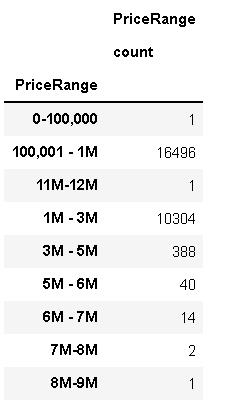
通过研究上表,可以得出以下结论:
- 1个数据项,范围0-100,00
- 7M-8M范围内有2个数据
- 8M-9M范围内有1个数据
- 11M-12M范围内有1个数据,
为了本研究的目的,让我们删除符合上述条件的行。
melbourne_data.info()

melbourne_data.describe().T

melbourne_data.drop(melbourne_data[(melbourne_data['PriceRange'] == '0-100,000') |
                                   (melbourne_data['PriceRange'] == '7M-8M') |
                                   (melbourne_data['PriceRange'] == '8M-9M') |
                                   (melbourne_data['PriceRange'] == '11M-12M')].index, inplace=True)

melbourne_data.describe().T

melbourne_data.groupby(['Rooms'])['Rooms'].count()

melbourne_data.drop(melbourne_data[(melbourne_data['Rooms'] == 12) |
                                   (melbourne_data['Rooms'] == 16)].index, inplace=True)

melbourne_data.describe().T
numerics = ['int16', 'int32', 'int64', 'float16', 'float32', 'float64']

melbourne_data.select_dtypes(include = numerics).hist(bins=15, figsize=(15, 6), layout=(2, 4))
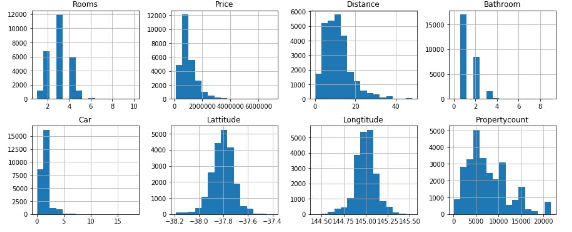
melbourne_data['Distance'] = round(melbourne_data['Distance'])

melbourne_data.shape
2 数据呈现与关系
2.1 我们考虑的第一个因素是价格与年份和季节的关系。然后利用线性函数预测2019年和2020年的价格。
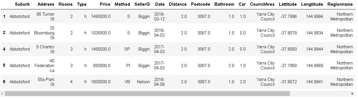
2.1.1 每种类型的房子价格年趋势
## 从日期中提取年出来
melbourne_data['Year']=melbourne_data['Date'].apply(lambda x:x.year)
melbourne_data.head(5)
# house
melbourne_data_h=melbourne_data[melbourne_data['Type']=='h']
# condo
melbourne_data_u=melbourne_data[melbourne_data['Type']=='u']
# townhouse
melbourne_data_t=melbourne_data[melbourne_data['Type']=='t']
# house,condo and townhouse price groupby year,求平均
melbourne_data_h_y=melbourne_data_h.groupby('Year').mean()
melbourne_data_u_y=melbourne_data_u.groupby('Year').mean()
melbourne_data_t_y=melbourne_data_t.groupby('Year').mean()
melbourne_data_h_y.head()

melbourne_data_h_y['Price'].plot(kind='line', color='r',label='House')
melbourne_data_u_y['Price'].plot(kind='line', color='g',label='Condo')
melbourne_data_t_y['Price'].plot(kind='line', color='b',label='Townhouse')
year_xticks=[2016,2017,2018]
plt.ylabel('Price')
plt.xticks(year_xticks)
plt.title('每种类型的房子价格年趋势')
plt.legend()
House大幅下跌10万套,Condo价格缓慢攀升,而Townhouse价格保持稳定。从这张图上可以看出,预计House会下降,但坡度较小的Townhouse房价会下降,不变的Condo价格会上升。对开发商来说,是时候在2019年建更多的公寓了。购房者的住房预算需要削减,是时候在2019年买房了。
2.2 预测2019年和2020年Southern Metropolitan所有类型的房屋、Southern Metropolitan的Condo和Eastern Metropolitan的Condo价格
melbourne_data.shape
melbourne_data.columns
melbourne_data_South_M=melbourne_data[melbourne_data['Regionname']=='Southern Metropolitan']
melbourne_data_South_M_average=melbourne_data_South_M.groupby(['Year'])['Price'].mean()

X = melbourne_data_South_M[[ 'Year']]
y = melbourne_data_South_M[['Price']]

lm2 = LinearRegression()
lm2.fit(X, y)

lm2.intercept_
lm2.coef_

X_new = pd.DataFrame({'Year': [2019,2020,2021]})

lm2.predict(X_new)

根据这一粗略估算,2019年和2020年墨尔本房屋平均价格将为1557639、1630019。
2.2.1 Southern Metropolitan的Condo价格预测
melbourne_data_SM=melbourne_data[melbourne_data['Regionname']=='Southern Metropolitan']
melbourne_data_SM_u=melbourne_data_SM[melbourne_data_SM['Type']=='u']
melbourne_data_SM_u.shape
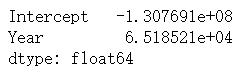
lm1 = smf.ols(formula='Price ~ Year', data=melbourne_data_SM_u).fit()

lm1.params

X_new = pd.DataFrame({'Year': [2016,2017,2018,2019,2020,2021]})

lm1.predict(X_new)

# 拟合度
lm1.rsquared
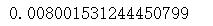
这拟合度,看看就得了。
2.2.2 Eastern Metropolitan的Condo价格预测
melbourne_data_E=melbourne_data[melbourne_data['Regionname']=='Eastern Metropolitan']
melbourne_data_E_u=melbourne_data_E[melbourne_data_E['Type']=='u']

lme = smf.ols(formula='Price ~ Year', data=melbourne_data_E_u).fit()

lme.params
melbourne_data_E_u.shape

X_new = pd.DataFrame({'Year': [2016,2017,2018,2019,2020,2021]})

lme.predict(X_new)
对于Eastern Metropolitan,预计2016年至2017年价格将增长10%,2018年至2019年价格将增长7.7%。虽然和南部地区相比,这个数字要少一些。
2.3 Seasonal performance
melbourne_data['Month']=pd.DatetimeIndex(melbourne_data['Date']).month

melbourne_data_2016=melbourne_data[melbourne_data['Year']==2016]
melbourne_data_2017=melbourne_data[melbourne_data['Year']==2017]
melbourne_data_2018=melbourne_data[melbourne_data['Year']==2018]
melbourne_data_2016_count=melbourne_data_2016.groupby(['Month']).count()
melbourne_data_2017_count=melbourne_data_2017.groupby(['Month']).count()
melbourne_data_2018_count=melbourne_data_2018.groupby(['Month']).count()
Comparison={2016:melbourne_data_2016.shape,2017:melbourne_data_2017.shape,2018:melbourne_data_2018.shape}
Comparison

label_2016=['January','March','April','May','June','July','August','September','October','November','December']
plt.pie(melbourne_data_2016_count['Price'],labels=label_2016,autopct='%.1f %%')
plt.title('Year 2016')
plt.show()
 Pandas Matplotlib:如何更改散点图中图例的形状和大小?