VRP问题基于模拟退火求解带时间窗的TWVRP问题
Posted 博主QQ2449341593
tags:
篇首语:本文由小常识网(cha138.com)小编为大家整理,主要介绍了VRP问题基于模拟退火求解带时间窗的TWVRP问题相关的知识,希望对你有一定的参考价值。
1. 简介
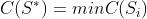
模拟退火算法的思想借鉴于固体的退火过程,当固体的温度很高时,内能比较大,固体内的粒子处于快速无序运动状态,当温度慢慢降低,固体的内能减小,粒子逐渐趋于有序,最终固体处于常温状态,内能达到最小,此时粒子最为稳定。
白话理解:一开始为算法设定一个较高的值T(模拟温度),算法不稳定,选择当前较差解的概率很大;随着T的减小,算法趋于稳定,选择较差解的概率减小,最后,T降至终止迭代的条件,得到近似最优解。
2.算法思想及步骤
设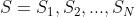 为所有的可能解,
 反映了取
反映了取 时解的代价,则组合优化问题可形式化地表述为寻找
使得
 。
。

其中,P为算法选择较差解的概率;T 为温度的模拟参数; 。
。
- 当T很大时,
 ,此时算法以较大概率选择非当前最优解;
 - P的值随着T的减小而减小;
- 当
 时,
时, ,此时算法几乎只选择最优解,等同于贪心算法。
带时间窗的车辆路径问题(VRPTW)
由于VRP问题的持续发展,考虑需求点对于车辆到达的时间有所要求之下,在车辆途程问题之中加入时窗的限制,便成为带时间窗车辆路径问题(VRP with Time Windows, VRPTW)。带时间窗车辆路径问题(VRPTW)是在VRP上加上了客户的被访问的时间窗约束。在VRPTW问题中,除了行驶成本之外, 成本函数还要包括由于早到某个客户而引起的等待时间和客户需要的服务时间。在VRPTW中,车辆除了要满足VRP问题的限制之外,还必须要满足需求点的时窗限制,而需求点的时窗限制可以分为两种,一种是硬时窗(Hard Time Window),硬时窗要求车辆必须要在时窗内到达,早到必须等待,而迟到则拒收;另一种是软时窗(Soft Time Window),不一定要在时窗内到达,但是在时窗之外到达必须要处罚,以处罚替代等待与拒收是软时窗与硬时窗最大的不同。
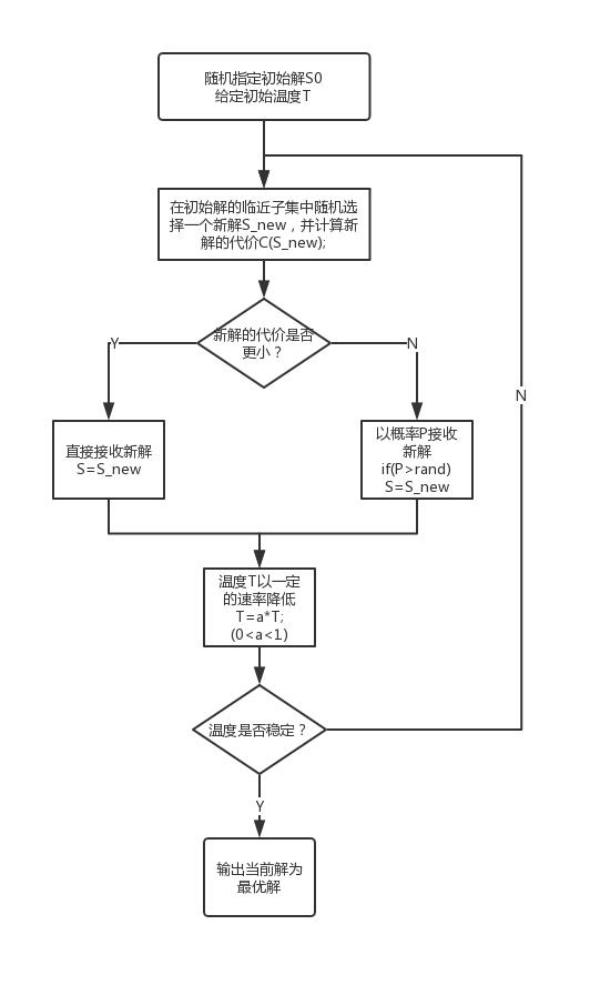
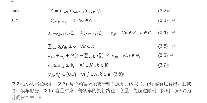
模型1问题定义:
The VRPTW is defined by a fleet of vehicles K={1,…,k} , a set of customers C={1,…,n} , and a directed graph G, Typically the fleet is considered to be homogeneous, that is, all vehicles are identical. The graph consists of |C| + 2 vertices, where the customers are denoted 1, 2,...,n and the depot is represented by the vertices 0 ("the starting depot") and n + 1 ("the returning depot"). The set of all vertices, that is, 0,1,... , n+1 is denoted N. The set of arcs, A, represents direct connections between the depot and the customers and among the customers. There are no arcs ending at vertex 0 or originating from vertex n + 1. With each arc (i,j), where i≠j , we associate a cost cij and a time tij , which may include service time at customer i.
Each vehicle has a capacity Q and each customer i a demand qi . Each customer i has a time window [ai,bi] and a vehicle must arrive at the customer before bi . If it arrives before the time window opens, it has to wait until ai to service the customer. The time windows for both depots are assumed to be identical to [a0,b0] which represents the scheduling horizon. The vehicles may not leave the depot before a0 and must return at the latest at time bn+1 .
It is assumed that Q, ai , bi , qi , cij are non-negative integers and tij are positive integers. Note that this assumption is necessary to develop an algorithm for the shortest path with resource constraints used in the column generation approach presented later. Furthermore it is assumed that the triangle inequality is satisfied for both cij and tij .
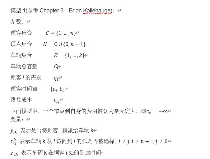
The decision variable s ik![]() is defined for each vertex i and each vehicle k and denotes the time vehicle k starts to service customer i. In case vehicle k does not service customer i, s ik
is defined for each vertex i and each vehicle k and denotes the time vehicle k starts to service customer i. In case vehicle k does not service customer i, s ik![]() has no meaning and consequently it's value is considered irrelevant. We assume a0 = 0 and therefore s 0k = 0, for all k.
has no meaning and consequently it's value is considered irrelevant. We assume a0 = 0 and therefore s 0k = 0, for all k.
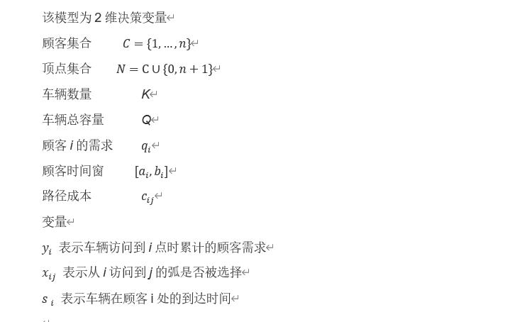
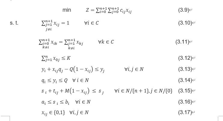
模型2(参考2017 A generalized formulation for vehicle routing problems):
该模型为2维决策变量

tic
clear
clc
%% 用importdata这个函数来读取文件
c101=importdata('c101.txt');
cap=200;
%% 提取数据信息
E=c101(1,5); %配送中心时间窗开始时间
L=c101(1,6); %配送中心时间窗结束时间
vertexs=c101(:,2:3); %所有点的坐标x和y
customer=vertexs(2:end,:); %顾客坐标
cusnum=size(customer,1); %顾客数
v_num=5; %车辆最多使用数目
demands=c101(2:end,4); %需求量
a=c101(2:end,5); %顾客时间窗开始时间[a[i],b[i]]
b=c101(2:end,6); %顾客时间窗结束时间[a[i],b[i]]
s=c101(2:end,7); %客户点的服务时间
h=pdist(vertexs);
dist=squareform(h); %距离矩阵
%% 模拟退火参数
belta=10; %违反的容量约束的惩罚函数系数
gama=100; %违反时间窗约束的惩罚函数系数
MaxOutIter=2000; %外层循环最大迭代次数
MaxInIter=300; %里层循环最大迭代次数
T0=100; %初始温度
alpha=0.99; %冷却因子
pSwap=0.2; %选择交换结构的概率
pReversion=0.5; %选择逆转结构的概率
pInsertion=1-pSwap-pReversion; %选择插入结构的概率
N=cusnum+v_num-1; %解长度=顾客数目+车辆最多使用数目-1
%% 随机构造初始解
currS=randperm(N); %随机构造初始解
[currVC,NV,TD,violate_num,violate_cus]=decode(currS,cusnum,cap,demands,a,b,L,s,dist); %对初始解解码
%求初始配送方案的成本=车辆行驶总成本+belta*违反的容量约束之和+gama*违反时间窗约束之和
currCost=costFuction(currVC,a,b,s,L,dist,demands,cap,belta,gama);
Sbest=currS; %初始将全局最优解赋值为初始解
bestVC=currVC; %初始将全局最优配送方案赋值为初始配送方案
bestCost=currCost; %初始将全局最优解的总成本赋值为初始解总成本
BestCost=zeros(MaxOutIter,1); %记录每一代全局最优解的总成本
T=T0; %温度初始化
%% 模拟退火
for outIter=1:MaxOutIter
for inIter=1:MaxInIter
newS=Neighbor(currS,pSwap,pReversion,pInsertion); %经过邻域结构后产生的新的解
%对新解解码=车辆行驶总成本+belta*违反的容量约束之和+gama*违反时间窗约束之和
newVC=decode(newS,cusnum,cap,demands,a,b,L,s,dist);
newCost=costFuction(newVC,a,b,s,L,dist,demands,cap,belta,gama); %求初始配送方案的成本
%如果新解比当前解更好,则更新当前解,以及当前解的总成本
if newCost<=currCost
currS=newS;
currVC=newVC;
currCost=newCost;
else
%如果新解不如当前解好,则采用退火准则,以一定概率接受新解
delta=(newCost-currCost)/currCost; %计算新解与当前解总成本相差的百分比
P=exp(-delta/T); %计算接受新解的概率
%如果0~1的随机数小于P,则接受新解,并更新当前解,以及当前解总成本
if rand<=P
currS=newS;
currVC=newVC;
currCost=newCost;
end
end
%将当前解与全局最优解进行比较,如果当前解更好,则更新全局最优解,以及全局最优解总成本
if currCost<=bestCost
Sbest=currS;
bestVC=currVC;
bestCost=currCost;
end
end
%记录外层循环每次迭代的全局最优解的总成本
BestCost(outIter)=bestCost;
%显示外层循环每次迭代的信全局最优解的总成本
disp(['第',num2str(outIter),'代全局最优解:'])
[bestVC,bestNV,bestTD,best_vionum,best_viocus]=decode(Sbest,cusnum,cap,demands,a,b,L,s,dist); %对全局最优解解码
disp(['车辆使用数目:',num2str(bestNV),',车辆行驶总距离:',num2str(bestTD),',违反约束路径数目:',num2str(best_vionum),',违反约束顾客数目:',num2str(best_viocus)]);
fprintf('\\n')
%更新当前温度
T=alpha*T;
end
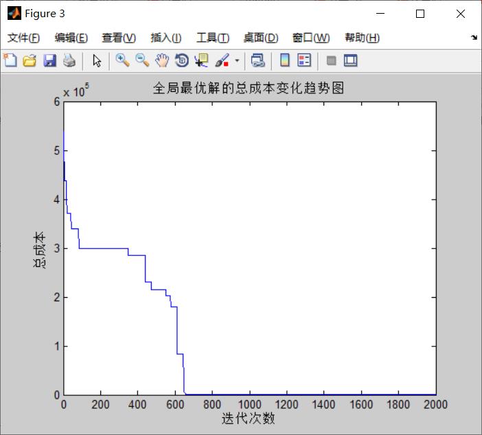
%% 打印外层循环每次迭代的全局最优解的总成本变化趋势图
figure;
plot(BestCost,'LineWidth',1);
title('全局最优解的总成本变化趋势图')
xlabel('迭代次数');
ylabel('总成本');
%% 打印全局最优解路线图
draw_Best(bestVC,vertexs);
toc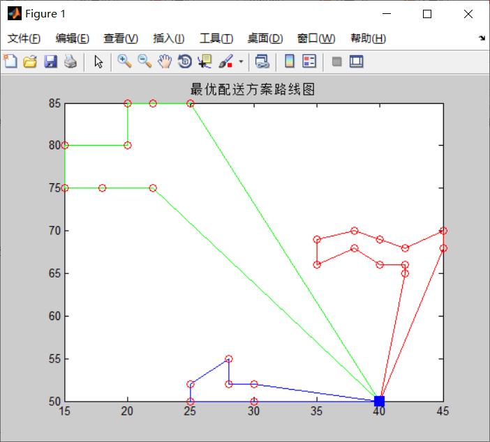
以上是关于VRP问题基于模拟退火求解带时间窗的TWVRP问题的主要内容,如果未能解决你的问题,请参考以下文章