L1,L2正则化本质
Posted
tags:
篇首语:本文由小常识网(cha138.com)小编为大家整理,主要介绍了L1,L2正则化本质相关的知识,希望对你有一定的参考价值。
参考技术A 经验风险其实就是样本本身带来的误差。结构风险就是学习器带来的误差。
当假设空间、损失函数、训练集确定的情况下,经验风险可以确定;
如果样本量足够大,经验风险趋近于期望损失,经验风险最小化可以保证有很好的学习效果;
但是如果样本量小,经验风险最小化的效果未必好,容易造成过拟合,因此结构最小化是为了防止过拟合而提出来的策略。
正则化是结构风险最小化策略的实现。
正则化符合奥卡姆剃刀原理:在所有可能选择的模型,能够很好的解释已知数据并且十分简单才是最好的模型
从贝叶斯估计的角度来看,正则化对应于模型的先验概率,可以假设复杂的模型有较大的先验概率,简单的模型有较小的先验概率。
有正则化就是最大后验概率的参数估计方法
无正则化就是最大似然概率的参数估计方法
先验概率,后验概率,似然概率,条件概率,贝叶斯,最大似然
似然函数,最大似然估计
f(x|θ)表示的就是在给定参数theta的情况下,x出现的可能性多大。L(θ|x)表示的是在给定样本x的时候,哪个参数theta使得x出现的可能性多大。
最大似然估计和最大后验概率估计的区别
相信读完上文,MLE和MAP的区别应该是很清楚的了。MAP就是多个作为因子的先验概率P(θ)。或者,也可以反过来,认为MLE是把先验概率P(θ)认为等于1,即认为θ是均匀分布。
详解最大似然估计(MLE)、最大后验概率估计(MAP),以及贝叶斯公式的理解
L1正则化产生稀疏的权值, L2正则化产生平滑的权值
L1也可以作为特征选择的一种
可以从两个角度解释:贝叶斯角度和梯度下降角度
常见的L1/L2正则,分别等价于引入先验信息:参数符合拉普拉斯分布/高斯分布。没有加,就是符合均匀分布
正则化以及优化
权重的初始化:
1.如果激活函数是:Relu: W(n[L],n[L-1])=np.random.rand(n[L],n[L-1]) *np.sqrt(2/n[L-1])
2.如果激活函数是:tanh: W(n[L],n[L-1])=np.random.rand(n[L],n[L-1]) *np.sqrt(1/n[L-1])
 1 def initialize_parameters_he(layers_dims):
 2     """
 3     Arguments:
 4     layer_dims -- python array (list) containing the size of each layer.
 5
 6     Returns:
 7     parameters -- python dictionary containing your parameters "W1", "b1", ..., "WL", "bL":
 8                     W1 -- weight matrix of shape (layers_dims[1], layers_dims[0])
 9                     b1 -- bias vector of shape (layers_dims[1], 1)
10                     ...
11                     WL -- weight matrix of shape (layers_dims[L], layers_dims[L-1])
12                     bL -- bias vector of shape (layers_dims[L], 1)
13     """
14
15     np.random.seed(3)
16     parameters = {}
17     L = len(layers_dims) - 1 # integer representing the number of layers
18
19     for l in range(1, L + 1):
20         ### START CODE HERE ### (≈ 2 lines of code)
21         parameters[‘W‘ + str(l)] = np.random.randn(layers_dims[l],layers_dims[l-1])*np.sqrt(1/layers_dims[l-1])
22         parameters[‘b‘ + str(l)] = np.zeros((layers_dims[l],1))
23         ### END CODE HERE ###
24
25     return parameters
正则化:
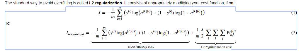
L2 Regularization : The standard way to avoid overfitting
1. Basic function:
  1 import numpy as np
  2 import matplotlib.pyplot as plt
  3 import h5py
  4 import sklearn
  5 import sklearn.datasets
  6 import sklearn.linear_model
  7 import scipy.io
  8
  9 def sigmoid(x):
 10     """
 11     Compute the sigmoid of x
 12
 13     Arguments:
 14     x -- A scalar or numpy array of any size.
 15
 16     Return:
 17     s -- sigmoid(x)
 18     """
 19     s = 1/(1+np.exp(-x))
 20     return s
 21
 22 def relu(x):
 23     """
 24     Compute the relu of x
 25
 26     Arguments:
 27     x -- A scalar or numpy array of any size.
 28
 29     Return:
 30     s -- relu(x)
 31     """
 32     s = np.maximum(0,x)
 33
 34     return s
 35
 36 def load_planar_dataset(seed):
 37
 38     np.random.seed(seed)
 39
 40     m = 400 # number of examples
 41     N = int(m/2) # number of points per class
 42     D = 2 # dimensionality
 43     X = np.zeros((m,D)) # data matrix where each row is a single example
 44     Y = np.zeros((m,1), dtype=‘uint8‘) # labels vector (0 for red, 1 for blue)
 45     a = 4 # maximum ray of the flower
 46
 47     for j in range(2):
 48         ix = range(N*j,N*(j+1))
 49         t = np.linspace(j*3.12,(j+1)*3.12,N) + np.random.randn(N)*0.2 # theta
 50         r = a*np.sin(4*t) + np.random.randn(N)*0.2 # radius
 51         X[ix] = np.c_[r*np.sin(t), r*np.cos(t)]
 52         Y[ix] = j
 53
 54     X = X.T
 55     Y = Y.T
 56
 57     return X, Y
 58
 59 def initialize_parameters(layer_dims):
 60     """
 61     Arguments:
 62     layer_dims -- python array (list) containing the dimensions of each layer in our network
 63
 64     Returns:
 65     parameters -- python dictionary containing your parameters "W1", "b1", ..., "WL", "bL":
 66                     W1 -- weight matrix of shape (layer_dims[l], layer_dims[l-1])
 67                     b1 -- bias vector of shape (layer_dims[l], 1)
 68                     Wl -- weight matrix of shape (layer_dims[l-1], layer_dims[l])
 69                     bl -- bias vector of shape (1, layer_dims[l])
 70
 71     Tips:
 72     - For example: the layer_dims for the "Planar Data classification model" would have been [2,2,1].
 73     This means W1‘s shape was (2,2), b1 was (1,2), W2 was (2,1) and b2 was (1,1). Now you have to generalize it!
 74     - In the for loop, use parameters[‘W‘ + str(l)] to access Wl, where l is the iterative integer.
 75     """
 76
 77     np.random.seed(3)
 78     parameters = {}
 79     L = len(layer_dims) # number of layers in the network
 80
 81     for l in range(1, L):
 82         parameters[‘W‘ + str(l)] = np.random.randn(layer_dims[l], layer_dims[l-1]) / np.sqrt(layer_dims[l-1])
 83         parameters[‘b‘ + str(l)] = np.zeros((layer_dims[l], 1))
 84
 85         assert(parameters[‘W‘ + str(l)].shape == layer_dims[l], layer_dims[l-1])
 86         assert(parameters[‘W‘ + str(l)].shape == layer_dims[l], 1)
 87
 88
 89     return parameters
 90
 91 def forward_propagation(X, parameters):
 92     """
 93     Implements the forward propagation (and computes the loss) presented in Figure 2.
 94
 95     Arguments:
 96     X -- input dataset, of shape (input size, number of examples)
 97     parameters -- python dictionary containing your parameters "W1", "b1", "W2", "b2", "W3", "b3":
 98                     W1 -- weight matrix of shape ()
 99                     b1 -- bias vector of shape ()
100                     W2 -- weight matrix of shape ()
101                     b2 -- bias vector of shape ()
102                     W3 -- weight matrix of shape ()
103                     b3 -- bias vector of shape ()
104
105     Returns:
106     loss -- the loss function (vanilla logistic loss)
107     """
108
109     # retrieve parameters
110     W1 = parameters["W1"]
111     b1 = parameters["b1"]
112     W2 = parameters["W2"]
113     b2 = parameters["b2"]
114     W3 = parameters["W3"]
115     b3 = parameters["b3"]
116
117     # LINEAR -> RELU -> LINEAR -> RELU -> LINEAR -> SIGMOID
118     Z1 = np.dot(W1, X) + b1
119     A1 = relu(Z1)
120     Z2 = np.dot(W2, A1) + b2
121     A2 = relu(Z2)
122     Z3 = np.dot(W3, A2) + b3
123     A3 = sigmoid(Z3)
124
125     cache = (Z1, A1, W1, b1, Z2, A2, W2, b2, Z3, A3, W3, b3)
126
127     return A3, cache
128
129 def backward_propagation(X, Y, cache):
130     """
131     Implement the backward propagation presented in figure 2.
132
133     Arguments:
134     X -- input dataset, of shape (input size, number of examples)
135     Y -- true "label" vector (containing 0 if cat, 1 if non-cat)
136     cache -- cache output from forward_propagation()
137
138     Returns:
139     gradients -- A dictionary with the gradients with respect to each parameter, activation and pre-activation variables
140     """
141     m = X.shape[1]
142     (Z1, A1, W1, b1, Z2, A2, W2, b2, Z3, A3, W3, b3) = cache
143
144     dZ3 = A3 - Y
145     dW3 = 1./m * np.dot(dZ3, A2.T)
146     db3 = 1./m * np.sum(dZ3, axis=1, keepdims = True)
147
148     dA2 = np.dot(W3.T, dZ3)
149     dZ2 = np.multiply(dA2, np.int64(A2 > 0))
150     dW2 = 1./m * np.dot(dZ2, A1.T)
151     db2 = 1./m * np.sum(dZ2, axis=1, keepdims = True)
152
153     dA1 = np.dot(W2.T, dZ2)
154     dZ1 = np.multiply(dA1, np.int64(A1 > 0))
155     dW1 = 1./m * np.dot(dZ1, X.T)
156     db1 = 1./m * np.sum(dZ1, axis=1, keepdims = True)
157
158     gradients = {"dZ3": dZ3, "dW3": dW3, "db3": db3,
159                  "dA2": dA2, "dZ2": dZ2, "dW2": dW2, "db2": db2,
160                  "dA1": dA1, "dZ1": dZ1, "dW1": dW1, "db1": db1}
161
162     return gradients
163
164 def update_parameters(parameters, grads, learning_rate):
165     """
166     Update parameters using gradient descent
167
168     Arguments:
169     parameters -- python dictionary containing your parameters:
170                     parameters[‘W‘ + str(i)] = Wi
171                     parameters[‘b‘ + str(i)] = bi
172     grads -- python dictionary containing your gradients for each parameters:
173                     grads[‘dW‘ + str(i)] = dWi
174                     grads[‘db‘ + str(i)] = dbi
175     learning_rate -- the learning rate, scalar.
176
177     Returns:
178     parameters -- python dictionary containing your updated parameters
179     """
180
181     n = len(parameters) // 2 # number of layers in the neural networks
182
183     # Update rule for each parameter
184     for k in range(n):
185         parameters["W" + str(k+1)] = parameters["W" + str(k+1)] - learning_rate * grads["dW" + str(k+1)]
186         parameters["b" + str(k+1)] = parameters["b" + str(k+1)] - learning_rate * grads["db" + str(k+1)]
187
188     return parameters
189
190 def predict(X, y, parameters):
191     """
192     This function is used to predict the results of a  n-layer neural network.
193
194     Arguments:
195     X -- data set of examples you would like to label
196     parameters -- parameters of the trained model
197
198     Returns:
199     p -- predictions for the given dataset X
200     """
201
202     m = X.shape[1]
203     p = np.zeros((1,m), dtype = np.int)
204
205     # Forward propagation
206     a3, caches = forward_propagation(X, parameters)
207
208     # convert probas to 0/1 predictions
209     for i in range(0, a3.shape[1]):
210         if a3[0,i] > 0.5:
211             p[0,i] = 1
212         else:
213             p[0,i] = 0
214
215     # print results
216
217     #print ("predictions: " + str(p[0,:]))
218     #print ("true labels: " + str(y[0,:]))
219     print("Accuracy: "  + str(np.mean((p[0,:] == y[0,:]))))
220
221     return p
222
223 def compute_cost(a3, Y):
224     """
225     Implement the cost function
226
227     Arguments:
228     a3 -- post-activation, output of forward propagation
229     Y -- "true" labels vector, same shape as a3
230
231     Returns:
232     cost - value of the cost function
233     """
234     m = Y.shape[1]
235
236     logprobs = np.multiply(-np.log(a3),Y) + np.multiply(-np.log(1 - a3), 1 - Y)
237     cost = 1./m * np.nansum(logprobs)
238
239     return cost
240
241 def load_dataset():
242     train_dataset = h5py.File(‘datasets/train_catvnoncat.h5‘, "r")
243     train_set_x_orig = np.array(train_dataset["train_set_x"][:]) # your train set features
244     train_set_y_orig = np.array(train_dataset["train_set_y"][:]) # your train set labels
245
246     test_dataset = h5py.File(‘datasets/test_catvnoncat.h5‘, "r")
247     test_set_x_orig = np.array(test_dataset["test_set_x"][:]) # your test set features
248     test_set_y_orig = np.array(test_dataset["test_set_y"][:]) # your test set labels
249
250     classes = np.array(test_dataset["list_classes"][:]) # the list of classes
251
252     train_set_y = train_set_y_orig.reshape((1, train_set_y_orig.shape[0]))
253     test_set_y = test_set_y_orig.reshape((1, test_set_y_orig.shape[0]))
254
255     train_set_x_orig = train_set_x_orig.reshape(train_set_x_orig.shape[0], -1).T
256     test_set_x_orig = test_set_x_orig.reshape(test_set_x_orig.shape[0], -1).T
257
258     train_set_x = train_set_x_orig/255
259     test_set_x = test_set_x_orig/255
260
261     return train_set_x, train_set_y, test_set_x, test_set_y, classes
262
263
264 def predict_dec(parameters, X):
265     """
266     Used for plotting decision boundary.
267
268     Arguments:
269     parameters -- python dictionary containing your parameters
270     X -- input data of size (m, K)
271
272     Returns
273     predictions -- vector of predictions of our model (red: 0 / blue: 1)
274     """
275
276     # Predict using forward propagation and a classification threshold of 0.5
277     a3, cache = forward_propagation(X, parameters)
278     predictions = (a3>0.5)
279     return predictions
280
281 def load_planar_dataset(randomness, seed):
282
283     np.random.seed(seed)
284
285     m = 50
286     N = int(m/2) # number of points per class
287     D = 2 # dimensionality
288     X = np.zeros((m,D)) # data matrix where each row is a single example
289     Y = np.zeros((m,1), dtype=‘uint8‘) # labels vector (0 for red, 1 for blue)
290     a = 2 # maximum ray of the flower
291
292     for j in range(2):
293
294         ix = range(N*j,N*(j+1))
295         if j == 0:
296             t = np.linspace(j, 4*3.1415*(j+1),N) #+ np.random.randn(N)*randomness # theta
297             r = 0.3*np.square(t) + np.random.randn(N)*randomness # radius
298         if j == 1:
299             t = np.linspace(j, 2*3.1415*(j+1),N) #+ np.random.randn(N)*randomness # theta
300             r = 0.2*np.square(t) + np.random.randn(N)*randomness # radius
301
302         X[ix] = np.c_[r*np.cos(t), r*np.sin(t)]
303         Y[ix] = j
304
305     X = X.T
306     Y = Y.T
307
308     return X, Y
309
310 def plot_decision_boundary(model, X, y):
311     # Set min and max values and give it some padding
312     x_min, x_max = X[0, :].min() - 1, X[0, :].max() + 1
313     y_min, y_max = X[1, :].min() - 1, X[1, :].max() + 1
314     h = 0.01
315     # Generate a grid of points with distance h between them
316     xx, yy = np.meshgrid(np.arange(x_min, x_max, h), np.arange(y_min, y_max, h))
317     # Predict the function value for the whole grid
318     Z = model(np.c_[xx.ravel(), yy.ravel()])
319     Z = Z.reshape(xx.shape)
320     # Plot the contour and training examples
321     plt.contourf(xx, yy, Z, cmap=plt.cm.Spectral)
322     plt.ylabel(‘x2‘)
323     plt.xlabel(‘x1‘)
324     plt.scatter(X[0, :], X[1, :], c=np.squeeze(y), cmap=plt.cm.Spectral)
325     plt.show()
326
327 def load_2D_dataset():
328     data = scipy.io.loadmat(‘datasets/data.mat‘)
329     train_X = data[‘X‘].T
330     train_Y = data[‘y‘].T
331     test_X = data[‘Xval‘].T
332     test_Y = data[‘yval‘].T
333
334     #plt.scatter(train_X[0, :], train_X[1, :], c=np.squeeze(train_Y), s=40, cmap=plt.cm.Spectral);
335
336     return train_X, train_Y, test_X, test_Y
2. Build Model
 1 def model(X, Y, learning_rate = 0.3, num_iterations = 30000, print_cost = True, lambd = 0, keep_prob = 1):
 2     """
 3     Implements a three-layer neural network: LINEAR->RELU->LINEAR->RELU->LINEAR->SIGMOID.
 4
 5     Arguments:
 6     X -- input data, of shape (input size, number of examples)
 7     Y -- true "label" vector (1 for blue dot / 0 for red dot), of shape (output size, number of examples)
 8     learning_rate -- learning rate of the optimization
 9     num_iterations -- number of iterations of the optimization loop
10     print_cost -- If True, print the cost every 10000 iterations
11     lambd -- regularization hyperparameter, scalar
12     keep_prob - probability of keeping a neuron active during drop-out, scalar.
13
14     Returns:
15     parameters -- parameters learned by the model. They can then be used to predict.
16     """
17
18     grads = {}
19     costs = []                            # to keep track of the cost
20     m = X.shape[1]                        # number of examples
21     layers_dims = [X.shape[0], 20, 3, 1]
22
23     # Initialize parameters dictionary.
24     parameters = initialize_parameters(layers_dims)
25
26     # Loop (gradient descent)
27
28     for i in range(0, num_iterations):
29
30         # Forward propagation: LINEAR -> RELU -> LINEAR -> RELU -> LINEAR -> SIGMOID.
31         if keep_prob == 1:
32             a3, cache = forward_propagation(X, parameters)
33         elif keep_prob < 1:
34             a3, cache = forward_propagation_with_dropout(X, parameters, keep_prob)
35
36         # Cost function
37         if lambd == 0:
38             cost = compute_cost(a3, Y)
39         else:
40             cost = compute_cost_with_regularization(a3, Y, parameters, lambd)
41
42         # Backward propagation.
43         assert(lambd==0 or keep_prob==1)    # it is possible to use both L2 regularization and dropout,
44                                             # but this assignment will only explore one at a time
45         if lambd == 0 and keep_prob == 1:
46             grads = backward_propagation(X, Y, cache)
47         elif lambd != 0:
48             grads = backward_propagation_with_regularization(X, Y, cache, lambd)
49         elif keep_prob < 1:
50             grads = backward_propagation_with_dropout(X, Y, cache, keep_prob)
51
52         # Update parameters.
53         parameters = update_parameters(parameters, grads, learning_rate)
54
55         # Print the loss every 10000 iterations
56         if print_cost and i % 10000 == 0:
57             print("Cost after iteration {}: {}".format(i, cost))
58         if print_cost and i % 1000 == 0:
59             costs.append(cost)
60
61     # plot the cost
62     plt.plot(costs)
63     plt.ylabel(‘cost‘)
64     plt.xlabel(‘iterations (x1,000)‘)
65     plt.title("Learning rate =" + str(learning_rate))
66     plt.show()
67
68     return parameters
3. Build without any regularzation
 1 parameters = model(train_X, train_Y)
 2 print ("On the training set:")
 3 predictions_train = predict(train_X, train_Y, parameters)
 4 print ("On the test set:")
 5 predictions_test = predict(test_X, test_Y, parameters)
 6 plt.title("Model without regularization")
 7 axes = plt.gca()
 8 axes.set_xlim([-0.75,0.40])
 9 axes.set_ylim([-0.75,0.65])
10 plot_decision_boundary(lambda x: predict_dec(parameters, x.T), train_X, train_Y)
4. Build model with L2 regularzation:
 1 #L2 regularization compute_cost function:
 2
 3 def compute_cost_with_regularization(A3, Y, parameters, lambd):
 4     """
 5     Implement the cost function with L2 regularization. See formula (2) above.
 6
 7     Arguments:
 8     A3 -- post-activation, output of forward propagation, of shape (output size, number of examples)
 9     Y -- "true" labels vector, of shape (output size, number of examples)
10     parameters -- python dictionary containing parameters of the model
11
12     Returns:
13     cost - value of the regularized loss function (formula (2))
14     """
15     m = Y.shape[1]
16     W1 = parameters["W1"]
17     W2 = parameters["W2"]
18     W3 = parameters["W3"]
19
20     cross_entropy_cost = compute_cost(A3, Y) # This gives you the cross-entropy part of the cost
21
22     ### START CODE HERE ### (approx. 1 line)
23     L2_regularization_cost = (1.0/(2*m))*lambd*(np.sum(np.square(W1))+np.sum(np.square(W2))+np.sum(np.square(W3)))
24     ### END CODER HERE ###
25
26     cost = cross_entropy_cost + L2_regularization_cost
27
28     return cost
29
30 # L2 backward_propagation regularization:
31
32 def backward_propagation_with_regularization(X, Y, cache, lambd):
33     """
34     Implements the backward propagation of our baseline model to which we added an L2 regularization.
35
36     Arguments:
37     X -- input dataset, of shape (input size, number of examples)
38     Y -- "true" labels vector, of shape (output size, number of examples)
39     cache -- cache output from forward_propagation()
40     lambd -- regularization hyperparameter, scalar
41
42     Returns:
43     gradients -- A dictionary with the gradients with respect to each parameter, activation and pre-activation variables
44     """
45
46     m = X.shape[1]
47     (Z1, A1, W1, b1, Z2, A2, W2, b2, Z3, A3, W3, b3) = cache
48
49     dZ3 = A3 - Y
50
51     ### START CODE HERE ### (approx. 1 line)
52     dW3 = 1./m * np.dot(dZ3, A2.T) + (lambd/m)*W3
53     ### END CODE HERE ###
54     db3 = 1./m * np.sum(dZ3, axis=1, keepdims = True)
55
56     dA2 = np.dot(W3.T, dZ3)
57     dZ2 = np.multiply(dA2, np.int64(A2 > 0))
58     ### START CODE HERE ### (approx. 1 line)
59     dW2 = 1./m * np.dot(dZ2, A1.T) + (lambd/m)*W2
60     ### END CODE HERE ###
61     db2 = 1./m * np.sum(dZ2, axis=1, keepdims = True)
62
63     dA1 = np.dot(W2.T, dZ2)
64     dZ1 = np.multiply(dA1, np.int64(A1 > 0))
65     ### START CODE HERE ### (approx. 1 line)
66     dW1 = 1./m * np.dot(dZ1, X.T) + (lambd/m)*W1
67     ### END CODE HERE ###
68     db1 = 1./m * np.sum(dZ1, axis=1, keepdims = True)
69
70     gradients = {"dZ3": dZ3, "dW3": dW3, "db3": db3,"dA2": dA2,
71                  "dZ2": dZ2, "dW2": dW2, "db2": db2, "dA1": dA1,
72                  "dZ1": dZ1, "dW1": dW1, "db1": db1}
73
74     return gradients
75
76 #Build with L2 regularization model:
77 parameters = model(train_X, train_Y, lambd = 0.7)
78 print ("On the train set:")
79 predictions_train = predict(train_X, train_Y, parameters)
80 print ("On the test set:")
81 predictions_test = predict(test_X, test_Y, parameters)
82 plt.title("Model with L2-regularization")
83 axes = plt.gca()
84 axes.set_xlim([-0.75,0.40])
85 axes.set_ylim([-0.75,0.65])
86 plot_decision_boundary(lambda x: predict_dec(parameters, x.T), train_X, train_Y)
Observations:
- The value of λ is a hyperparameter that you can tune using a dev set.
- L2 regularization makes your decision boundary smoother. If λ is too large, it is also possible to "oversmooth", resulting in a model with high bias.
What is L2-regularization actually doing?:
L2-regularization relies on the assumption that a model with small weights is simpler than a model with large weights. Thus, by penalizing the square values of the weights in the cost function you drive all the weights to smaller values. It becomes too costly for the cost to have large weights! This leads to a smoother model in which the output changes more slowly as the input changes.
**What you should remember** -- the implications of L2-regularization on: - The cost computation: - A regularization term is added to the cost - The backpropagation function: - There are extra terms in the gradients with respect to weight matrices - Weights end up smaller ("weight decay"): - Weights are pushed to smaller values.
5. Build modle with Dropout
Dropout is a widely used regularization technique that is specific to deep learning. It randomly shuts down some neurons in each iteration,
You shut down each neuron of a layer with probability 1-keep_prob or keep it with probability keep_prob.The dropped neurons don‘t contribute to the training in both the forward and backward propagations of the iteration. When you shut some neurons down,you actually modify your model ,you train a different model that uses only a subset of your neurons.
5.1 Forward propagation with dropout:
We just add dropout to the hidden layers, not apply dropout to the input layer or output layer.
 1 def forward_propagation_with_dropout(X, parameters, keep_prob = 0.5):
 2     """
 3     Implements the forward propagation: LINEAR -> RELU + DROPOUT -> LINEAR -> RELU + DROPOUT -> LINEAR -> SIGMOID.
 4
 5     Arguments:
 6     X -- input dataset, of shape (2, number of examples)
 7     parameters -- python dictionary containing your parameters "W1", "b1", "W2", "b2", "W3", "b3":
 8                     W1 -- weight matrix of shape (20, 2)
 9                     b1 -- bias vector of shape (20, 1)
10                     W2 -- weight matrix of shape (3, 20)
11                     b2 -- bias vector of shape (3, 1)
12                     W3 -- weight matrix of shape (1, 3)
13                     b3 -- bias vector of shape (1, 1)
14     keep_prob - probability of keeping a neuron active during drop-out, scalar
15
16     Returns:
17     A3 -- last activation value, output of the forward propagation, of shape (1,1)
18     cache -- tuple, information stored for computing the backward propagation
19     """
20
21     np.random.seed(1)
22
23     # retrieve parameters
24     W1 = parameters["W1"]
25     b1 = parameters["b1"]
26     W2 = parameters["W2"]
27     b2 = parameters["b2"]
28     W3 = parameters["W3"]
29     b3 = parameters["b3"]
30
31     # LINEAR -> RELU -> LINEAR -> RELU -> LINEAR -> SIGMOID
32     Z1 = np.dot(W1, X) + b1
33     A1 = relu(Z1)
34     ### START CODE HERE ### (approx. 4 lines)         # Steps 1-4 below correspond to the Steps 1-4 described above.
35     D1 = np.random.rand(A1.shape[0],A1.shape[1])                                         # Step 1: initialize matrix D1 = np.random.rand(..., ...)
36     D1 = (D1<keep_prob)                                         # Step 2: convert entries of D1 to 0 or 1 (using keep_prob as the threshold)
37     A1 = A1*D1                                         # Step 3: shut down some neurons of A1
38     A1 = A1/keep_prob                                        # Step 4: scale the value of neurons that haven‘t been shut down
39     ### END CODE HERE ###
40     Z2 = np.dot(W2, A1) + b2
41     A2 = relu(Z2)
42     ### START CODE HERE ### (approx. 4 lines)
43     D2 = np.random.rand(A2.shape[0],A2.shape[1])                                         # Step 1: initialize matrix D2 = np.random.rand(..., ...)
44     D2 = (D2<keep_prob)                                         # Step 2: convert entries of D2 to 0 or 1 (using keep_prob as the threshold)
45     A2 = A2*D2                                         # Step 3: shut down some neurons of A2
46     A2 = A2/keep_prob                                         # Step 4: scale the value of neurons that haven‘t been shut down
47     ### END CODE HERE ###
48     Z3 = np.dot(W3, A2) + b3
49     A3 = sigmoid(Z3)
50
51     cache = (Z1, D1, A1, W1, b1, Z2, D2, A2, W2, b2, Z3, A3, W3, b3)
52
53     return A3, cache
5.2 Backward propagation with dropout:
 1 def backward_propagation_with_dropout(X, Y, cache, keep_prob):
 2     """
 3     Implements the backward propagation of our baseline model to which we added dropout.
 4
 5     Arguments:
 6     X -- input dataset, of shape (2, number of examples)
 7     Y -- "true" labels vector, of shape (output size, number of examples)
 8     cache -- cache output from forward_propagation_with_dropout()
 9     keep_prob - probability of keeping a neuron active during drop-out, scalar
10
11     Returns:
12     gradients -- A dictionary with the gradients with respect to each parameter, activation and pre-activation variables
13     """
14
15     m = X.shape[1]
16     (Z1, D1, A1, W1, b1, Z2, D2, A2, W2, b2, Z3, A3, W3, b3) = cache
17
18     dZ3 = A3 - Y
19     dW3 = 1./m * np.dot(dZ3, A2.T)
20     db3 = 1./m * np.sum(dZ3, axis=1, keepdims = True)
21     dA2 = np.dot(W3.T, dZ3)
22     ### START CODE HERE ### (≈ 2 lines of code)
23     dA2 = dA2*D2              # Step 1: Apply mask D2 to shut down the same neurons as during the forward propagation
24     dA2 = dA2/keep_prob             # Step 2: Scale the value of neurons that haven‘t been shut down
25     ### END CODE HERE ###
26     dZ2 = np.multiply(dA2, np.int64(A2 > 0))
27     dW2 = 1./m * np.dot(dZ2, A1.T)
28     db2 = 1./m * np.sum(dZ2, axis=1, keepdims = True)
29
30     dA1 = np.dot(W2.T, dZ2)
31     ### START CODE HERE ### (≈ 2 lines of code)
32     dA1 = dA1*D1              # Step 1: Apply mask D1 to shut down the same neurons as during the forward propagation
33     dA1 = dA1/keep_prob              # Step 2: Scale the value of neurons that haven‘t been shut down
34     ### END CODE HERE ###
35     dZ1 = np.multiply(dA1, np.int64(A1 > 0))
36     dW1 = 1./m * np.dot(dZ1, X.T)
37     db1 = 1./m * np.sum(dZ1, axis=1, keepdims = True)
38
39     gradients = {"dZ3": dZ3, "dW3": dW3, "db3": db3,"dA2": dA2,
40                  "dZ2": dZ2, "dW2": dW2, "db2": db2, "dA1": dA1,
41                  "dZ1": dZ1, "dW1": dW1, "db1": db1}
42
43     return gradients
5.3 Build model with dropout :
 1 parameters = model(train_X, train_Y, keep_prob = 0.86, learning_rate = 0.3)
 2
 3 print ("On the train set:")
 4 predictions_train = predict(train_X, train_Y, parameters)
 5 print ("On the test set:")
 6 predictions_test = predict(test_X, test_Y, parameters)
 7 plt.title("Model with dropout")
 8 axes = plt.gca()
 9 axes.set_xlim([-0.75,0.40])
10 axes.set_ylim([-0.75,0.65])
11 plot_decision_boundary(lambda x: predict_dec(parameters, x.T), train_X, train_Y)
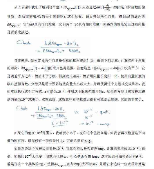
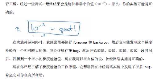
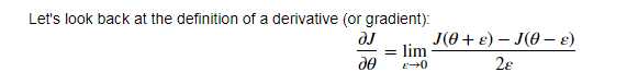
6. Gradient Checking:
f‘=(f(x+e)-f(x-e))/2e 双边误差 e逼近无穷小

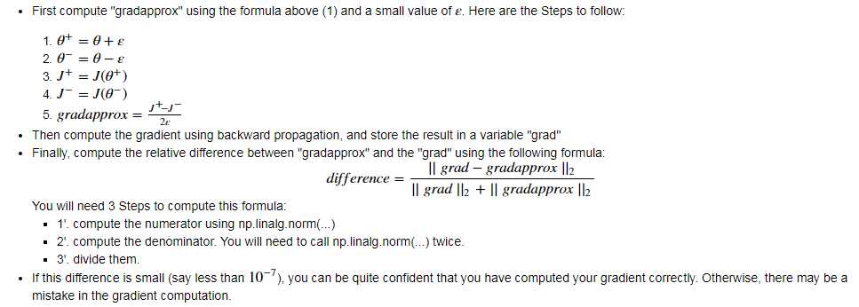
 1 #forward_propagation function
 2 def forward_propagation(x, theta):
 3     """
 4     Implement the linear forward propagation (compute J) presented in Figure 1 (J(theta) = theta * x)
 5
 6     Arguments:
 7     x -- a real-valued input
 8     theta -- our parameter, a real number as well
 9
10     Returns:
11     J -- the value of function J, computed using the formula J(theta) = theta * x
12     """
13
14     ### START CODE HERE ### (approx. 1 line)
15     J = np.multiply(x,theta)
16     ### END CODE HERE ###
17
18     return J
19
20 #backward_propagation function:
21
22 def backward_propagation(x, theta):
23     """
24     Computes the derivative of J with respect to theta (see Figure 1).
25
26     Arguments:
27     x -- a real-valued input
28     theta -- our parameter, a real number as well
29
30     Returns:
31     dtheta -- the gradient of the cost with respect to theta
32     """
33
34     ### START CODE HERE ### (approx. 1 line)
35     dtheta = x
36     ### END CODE HERE ###
37
38     return dtheta
39
40 #gradient_check function:
41 def gradient_check(x, theta, epsilon = 1e-7):
42     """
43     Implement the backward propagation presented in Figure 1.
44
45     Arguments:
46     x -- a real-valued input
47     theta -- our parameter, a real number as well
48     epsilon -- tiny shift to the input to compute approximated gradient with formula(1)
49
50     Returns:
51     difference -- difference (2) between the approximated gradient and the backward propagation gradient
52     """
53
54     # Compute gradapprox using left side of formula (1). epsilon is small enough, you don‘t need to worry about the limit.
55     ### START CODE HERE ### (approx. 5 lines)
56     thetaplus = theta+epsilon                             # Step 1
57     thetaminus = theta-epsilon                              # Step 2
58     J_plus = forward_propagation(x,thetaplus)                                  # Step 3
59     J_minus = forward_propagation(x,thetaminus)                                 # Step 4
60     gradapprox = (J_plus-J_minus)/(2*epsilon)                              # Step 5
61     ### END CODE HERE ###
62
63     # Check if gradapprox is close enough to the output of backward_propagation()
64     ### START CODE HERE ### (approx. 1 line)
65     grad = backward_propagation(x,theta)
66     ### END CODE HERE ###
67
68     ### START CODE HERE ### (approx. 1 line)
69     numerator = np.linalg.norm(grad-gradapprox)                               # Step 1‘
70     denominator = np.linalg.norm(grad)+np.linalg.norm(gradapprox)                             # Step 2‘
71     difference = numerator/denominator                              # Step 3‘
72     ### END CODE HERE ###
73
74     if difference < 1e-7:
75         print ("The gradient is correct!")
76     else:
77         print ("The gradient is wrong!")
78
79     return difference
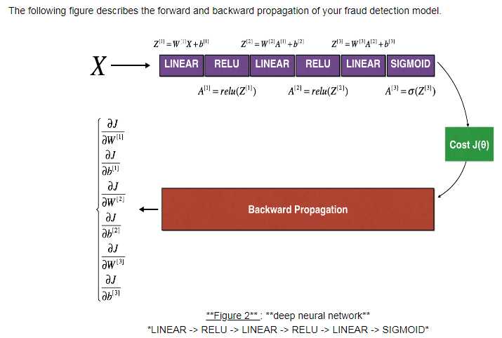
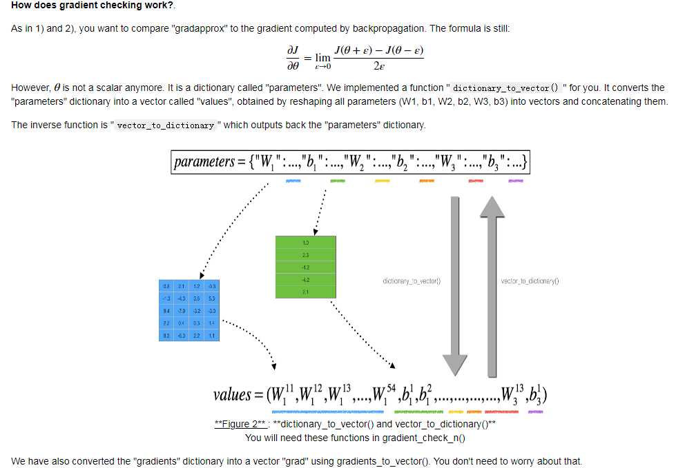
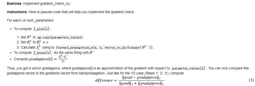
N-dimensional gradient checking:
以上是关于L1,L2正则化本质的主要内容,如果未能解决你的问题,请参考以下文章