Pytorch实战100例-第6天:好莱坞明星识别
Posted K同学啊
tags:
篇首语:本文由小常识网(cha138.com)小编为大家整理,主要介绍了Pytorch实战100例-第6天:好莱坞明星识别相关的知识,希望对你有一定的参考价值。

本文为🔗365天深度学习训练营 内部限免文章,参考本文所写记录性文章,请在文章开头注明以下内容,复制粘贴即可
- 🍨 本文为🔗365天深度学习训练营 中的学习记录博客
- 🍦 参考文章:Pytorch实战 | 第P6周:好莱坞明星识别
- 🍖 原作者:K同学啊|接辅导、项目定制
🍺要求:
- 保存训练过程中的最佳模型权重
- 调用官方的VGG-16网络框架
🍻拔高(可选):
- 测试集准确率达到60%(难度有点大,但是这个过程可以学到不少)
- 手动搭建VGG-16网络框架
🏡 我的环境:
- 语言环境:Python3.8
- 编译器:Jupyter Lab
- 深度学习环境:Pytorch
- torch==1.12.1+cu113
- torchvision==0.13.1+cu113
文章目录
一、 前期准备
1. 设置GPU
如果设备上支持GPU就使用GPU,否则使用CPU
import torch
import torch.nn as nn
import torchvision.transforms as transforms
import torchvision
from torchvision import transforms, datasets
import os,PIL,pathlib,warnings

warnings.filterwarnings("ignore")             #忽略警告信息

device = torch.device("cuda" if torch.cuda.is_available() else "cpu")
device
device(type='cuda')
2. 导入数据
import os,PIL,random,pathlib

data_dir = './6-data/'
data_dir = pathlib.Path(data_dir)

data_paths  = list(data_dir.glob('*'))
classeNames = [str(path).split("\\\\")[1] for path in data_paths]
classeNames
['Angelina Jolie',
 'Brad Pitt',
 'Denzel Washington',
 'Hugh Jackman',
 'Jennifer Lawrence',
 'Johnny Depp',
 'Kate Winslet',
 'Leonardo DiCaprio',
 'Megan Fox',
 'Natalie Portman',
 'Nicole Kidman',
 'Robert Downey Jr',
 'Sandra Bullock',
 'Scarlett Johansson',
 'Tom Cruise',
 'Tom Hanks',
 'Will Smith']
# 关于transforms.Compose的更多介绍可以参考:https://blog.csdn.net/qq_38251616/article/details/124878863
train_transforms = transforms.Compose([
    transforms.Resize([224, 224]),  # 将输入图片resize成统一尺寸
    # transforms.RandomHorizontalFlip(), # 随机水平翻转
    transforms.ToTensor(),          # 将PIL Image或numpy.ndarray转换为tensor,并归一化到[0,1]之间
    transforms.Normalize(           # 标准化处理-->转换为标准正太分布(高斯分布),使模型更容易收敛
        mean=[0.485, 0.456, 0.406],
        std=[0.229, 0.224, 0.225])  # 其中 mean=[0.485,0.456,0.406]与std=[0.229,0.224,0.225] 从数据集中随机抽样计算得到的。
])

test_transform = transforms.Compose([
    transforms.Resize([224, 224]),  # 将输入图片resize成统一尺寸
    transforms.ToTensor(),          # 将PIL Image或numpy.ndarray转换为tensor,并归一化到[0,1]之间
    transforms.Normalize(           # 标准化处理-->转换为标准正太分布(高斯分布),使模型更容易收敛
        mean=[0.485, 0.456, 0.406],
        std=[0.229, 0.224, 0.225])  # 其中 mean=[0.485,0.456,0.406]与std=[0.229,0.224,0.225] 从数据集中随机抽样计算得到的。
])

total_data = datasets.ImageFolder("./6-data/",transform=train_transforms)
total_data
Dataset ImageFolder
    Number of datapoints: 1800
    Root location: ./6-data/
    StandardTransform
Transform: Compose(
               Resize(size=[224, 224], interpolation=bilinear, max_size=None, antialias=None)
               ToTensor()
               Normalize(mean=[0.485, 0.456, 0.406], std=[0.229, 0.224, 0.225])
           )
total_data.class_to_idx
'Angelina Jolie': 0,
 'Brad Pitt': 1,
 'Denzel Washington': 2,
 'Hugh Jackman': 3,
 'Jennifer Lawrence': 4,
 'Johnny Depp': 5,
 'Kate Winslet': 6,
 'Leonardo DiCaprio': 7,
 'Megan Fox': 8,
 'Natalie Portman': 9,
 'Nicole Kidman': 10,
 'Robert Downey Jr': 11,
 'Sandra Bullock': 12,
 'Scarlett Johansson': 13,
 'Tom Cruise': 14,
 'Tom Hanks': 15,
 'Will Smith': 16
3. 划分数据集
train_size = int(0.8 * len(total_data))
test_size  = len(total_data) - train_size
train_dataset, test_dataset = torch.utils.data.random_split(total_data, [train_size, test_size])
train_dataset, test_dataset
(<torch.utils.data.dataset.Subset at 0x2570a8b6680>,
 <torch.utils.data.dataset.Subset at 0x2570a8b67a0>)
batch_size = 32

train_dl = torch.utils.data.DataLoader(train_dataset,
                                           batch_size=batch_size,
                                           shuffle=True,
                                           num_workers=1)
test_dl = torch.utils.data.DataLoader(test_dataset,
                                          batch_size=batch_size,
                                          shuffle=True,
                                          num_workers=1)
for X, y in test_dl:
    print("Shape of X [N, C, H, W]: ", X.shape)
    print("Shape of y: ", y.shape, y.dtype)
    break
Shape of X [N, C, H, W]:  torch.Size([32, 3, 224, 224])
Shape of y:  torch.Size([32]) torch.int64
二、调用官方的VGG-16模型
from torchvision.models import vgg16

device = "cuda" if torch.cuda.is_available() else "cpu"
print("Using  device".format(device))

# 加载预训练模型,并且对模型进行微调
model = vgg16(pretrained = True).to(device) # 加载预训练的vgg16模型

for param in model.parameters():
    param.requires_grad = False # 冻结模型的参数,这样子在训练的时候只训练最后一层的参数

# 修改classifier模块的第6层(即:(6): Linear(in_features=4096, out_features=2, bias=True))
# 注意查看我们下方打印出来的模型
model.classifier._modules['6'] = nn.Linear(4096,len(classeNames)) # 修改vgg16模型中最后一层全连接层,输出目标类别个数
model.to(device)
model
Using cuda device

VGG(
  (features): Sequential(
    (0): Conv2d(3, 64, kernel_size=(3, 3), stride=(1, 1), padding=(1, 1))
    (1): ReLU(inplace=True)
    (2): Conv2d(64, 64, kernel_size=(3, 3), stride=(1, 1), padding=(1, 1))
    (3): ReLU(inplace=True)
    (4): MaxPool2d(kernel_size=2, stride=2, padding=0, dilation=1, ceil_mode=False)
    (5): Conv2d(64, 128, kernel_size=(3, 3), stride=(1, 1), padding=(1, 1))
    (6): ReLU(inplace=True)
    (7): Conv2d(128, 128, kernel_size=(3, 3), stride=(1, 1), padding=(1, 1))
    (8): ReLU(inplace=True)
    (9): MaxPool2d(kernel_size=2, stride=2, padding=0, dilation=1, ceil_mode=False)
    (10): Conv2d(128, 256, kernel_size=(3, 3), stride=(1, 1), padding=(1, 1))
    (11): ReLU(inplace=True)
    (12): Conv2d(256, 256, kernel_size=(3, 3), stride=(1, 1), padding=(1, 1))
    (13): ReLU(inplace=True)
    (14): Conv2d(256, 256, kernel_size=(3, 3), stride=(1, 1), padding=(1, 1))
    (15): ReLU(inplace=True)
    (16): MaxPool2d(kernel_size=2, stride=2, padding=0, dilation=1, ceil_mode=False)
    (17): Conv2d(256, 512, kernel_size=(3, 3), stride=(1, 1), padding=(1, 1))
    (18): ReLU(inplace=True)
    (19): Conv2d(512, 512, kernel_size=(3, 3), stride=(1, 1), padding=(1, 1))
    (20): ReLU(inplace=True)
    (21): Conv2d(512, 512, kernel_size=(3, 3), stride=(1, 1), padding=(1, 1))
    (22): ReLU(inplace=True)
    (23): MaxPool2d(kernel_size=2, stride=2, padding=0, dilation=1, ceil_mode=False)
    (24): Conv2d(512, 512, kernel_size=(3, 3), stride=(1, 1), padding=(1, 1))
    (25): ReLU(inplace=True)
    (26): Conv2d(512, 512, kernel_size=(3, 3), stride=(1, 1), padding=(1, 1))
    (27): ReLU(inplace=True)
    (28): Conv2d(512, 512, kernel_size=(3, 3), stride=(1, 1), padding=(1, 1))
    (29): ReLU(inplace=True)
    (30): MaxPool2d(kernel_size=2, stride=2, padding=0, dilation=1, ceil_mode=False)
  )
  (avgpool): AdaptiveAvgPool2d(output_size=(7, 7))
  (classifier): Sequential(
    (0): Linear(in_features=25088, out_features=4096, bias=True)
    (1): ReLU(inplace=True)
    (2): Dropout(p=0.5, inplace=False)
    (3): Linear(in_features=4096, out_features=4096, bias=True)
    (4): ReLU(inplace=True)
    (5): Dropout(p=0.5, inplace=False)
    (6): Linear(in_features=4096, out_features=17, bias=True)
  )
)
三、 训练模型
1. 编写训练函数
# 训练循环
def train(dataloader, model, loss_fn, optimizer):
    size = len(dataloader.dataset)  # 训练集的大小
    num_batches = len(dataloader)   # 批次数目, (size/batch_size,向上取整)

    train_loss, train_acc = 0, 0  # 初始化训练损失和正确率

    for X, y in dataloader:  # 获取图片及其标签
        X, y = X.to(device), y.to(device)

        # 计算预测误差
        pred = model(X)          # 网络输出
        loss = loss_fn(pred, y)  # 计算网络输出和真实值之间的差距,targets为真实值,计算二者差值即为损失

        # 反向传播
        optimizer.zero_grad()  # grad属性归零
        loss.backward()        # 反向传播
        optimizer.step()       # 每一步自动更新

        # 记录acc与loss
        train_acc  += (pred.argmax(1) == y).type(torch.float).sum().item()
        train_loss += loss.item()

    train_acc  /= size
    train_loss /= num_batches

    return train_acc, train_loss
3. 编写测试函数
测试函数和训练函数大致相同,但是由于不进行梯度下降对网络权重进行更新,所以不需要传入优化器
def test (dataloader, model, loss_fn):
    size        = len(dataloader.dataset)  # 测试集的大小
    num_batches = len(dataloader)          # 批次数目, (size/batch_size,向上取整)
    test_loss, test_acc = 0, 0

    # 当不进行训练时,停止梯度更新,节省计算内存消耗
    with torch.no_grad():
        for imgs, target in dataloader:
            imgs, target = imgs.to(device), target.to(device)

            # 计算loss
            target_pred = model(imgs)
            loss        = loss_fn(target_pred, target)

            test_loss += loss.item()
            test_acc  += (target_pred.argmax(1) == target).type(torch.float).sum().item()

    test_acc  /= size
    test_loss /= num_batches

    return test_acc, test_loss
3. 设置动态学习率
# def adjust_learning_rate(optimizer, epoch, start_lr):
#     # 每 2 个epoch衰减到原来的 0.98
#     lr = start_lr * (0.92 ** (epoch // 2))
#     for param_group in optimizer.param_groups:
#         param_group['lr'] = lr

learn_rate = 1e-4 # 初始学习率
# optimizer  = torch.optim.SGD(model.parameters(), lr=learn_rate)
✨调用官方动态学习率接口
与上面方法是等价的
# 调用官方动态学习率接口时使用
lambda1 = lambda epoch: 0.92 ** (epoch // 4)
optimizer = torch.optim.SGD(model.parameters(), lr=learn_rate)
scheduler = torch.optim.lr_scheduler.LambdaLR(optimizer, lr_lambda=lambda1) #选定调整方法
👉调用官方接口示例:
model = [Parameter(torch.randn(2, 2, requires_grad=True))]
optimizer = SGD(model, 0.1)
scheduler = ExponentialLR(optimizer, gamma=0.9)

for epoch in range(20):
    for input, target in dataset:
        optimizer.zero_grad()
        output = model(input)
        loss = loss_fn(output, target)
        loss.backward()
        optimizer.step()
    scheduler.step()
更多的官方动态学习率设置方式可参考:https://pytorch.org/docs/stable/optim.html
4. 正式训练
model.train()、model.eval()训练营往期文章中有详细的介绍。
import copy

loss_fn    = nn.CrossEntropyLoss() # 创建损失函数
epochs     = 40

train_loss = []
train_acc  = []
test_loss  = []
test_acc   = []

best_acc = 0    # 设置一个最佳准确率,作为最佳模型的判别指标

for epoch in range(epochs):
    # 更新学习率(使用自定义学习率时使用)
    # adjust_learning_rate(optimizer, epoch, learn_rate)

    model.train()
    epoch_train_acc, epoch_train_loss = train(train_dl, model, loss_fn, optimizer)
    scheduler.step() # 更新学习率(调用官方动态学习率接口时使用)

    model.eval()
    epoch_test_acc, epoch_test_loss = test(test_dl, model, loss_fn)

    # 保存最佳模型到 best_model
    if epoch_test_acc > best_acc:
        best_acc   = epoch_test_acc
        best_model = copy.deepcopy(model)

    train_acc.append(epoch_train_acc)
    train_loss.append(epoch_train_loss)
    test_acc.append(epoch_test_acc)
    test_loss.append(epoch_test_loss)

    # 获取当前的学习率
    lr = optimizer.state_dict()['param_groups'][0]['lr']

    template = ('Epoch::2d, Train_acc::.1f%, Train_loss::.3f, Test_acc::.1f%, Test_loss::.3f, Lr::.2E')
    print(template.format(epoch+1, epoch_train_acc*100, epoch_train_loss,
                          epoch_test_acc*100, epoch_test_loss, lr))

# 保存最佳模型到文件中
PATH = './best_model.pth'  # 保存的参数文件名
torch.save(model.state_dict(), PATH)

print('Done')
Epoch: 1, Train_acc:6.2%, Train_loss:2.898, Test_acc:5.6%, Test_loss:2.845, Lr:1.00E-04
Epoch: 2, Train_acc:6.8%, Train_loss:2.873, Test_acc:7.8%, Test_loss:2.811, Lr:1.00E-04
Epoch: 3, Train_acc:8.1%, Train_loss:2.840, Test_acc:8.6%, Test_loss:2.811, Lr:1.00E-04
Epoch: 4, Train_acc:9.5%, Train_loss:2.798, Test_acc:13.6%, Test_loss:2.754, Lr:9.20E-05
.......
Epoch:38, Train_acc:18.1%, Train_loss:2.454, Test_acc:16.9%, Test_loss:2.471, Lr:4.72E-05
Epoch:39, Train_acc:20.6%, Train_loss:2.461, Test_acc:16.9%, Test_loss:2.476, Lr:4.72E-05
Epoch:40, Train_acc:20.3%, Train_loss:2.446, Test_acc:17.2%, Test_loss:2.458, Lr:4.34E-05
Done
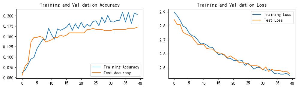
四、 结果可视化
1. Loss与Accuracy图
import matplotlib.pyplot as plt
#隐藏警告
import warnings
warnings.filterwarnings("ignore")               #忽略警告信息
plt.rcParams['font.sans-serif']    = ['SimHei'] # 用来正常显示中文标签
plt.rcParams['axes.unicode_minus'] = False      # 用来正常显示负号
plt.rcParams['figure.dpi']         = 100        #分辨率

epochs_range = range(epochs)

plt.figure(figsize=(12, 3))
plt.subplot(1, 2, 1)

plt.plot(epochs_range, train_acc, label='Training Accuracy')
plt.plot(epochs_range, test_acc, label='Test Accuracy')
plt.legend(loc='lower right')
plt.title('Training and Validation Accuracy')

plt.subplot(1, 2, 2)
plt.plot(epochs_range, train_loss, label='Training Loss')
plt.plot(epochs_range, test_loss, label='Test Loss')
plt.legend(loc='upper right')
plt.title('Training and Validation Loss')
plt.show()
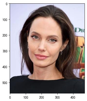
2. 指定图片进行预测
from PIL import Image

classes = list(total_data.class_to_idx)

def predict_one_image(image_path, model, transform, classes):

    test_img = Image.open(image_path).convert('RGB')
    plt.imshow(test_img)  # 展示预测的图片

    test_img = transform(test_img)
    img = test_img.to(device).unsqueeze(0)

    model.eval()
    output = model(img)

    _,pred = torch.max(output,1)
    pred_class = classes[pred]
    print(f'预测结果是:pred_class')
# 预测训练集中的某张照片
predict_one_image(image_path='./6-data/Angelina Jolie/001_fe3347c0.jpg',
                  model=model,
                  transform=train_transforms,
                  classes=classes)
预测结果是:Angelina Jolie
3. 模型评估
best_model.eval()
epoch_test_acc, epoch_test_loss = test(test_dl, best_model, loss_fn)
epoch_test_acc, epoch_test_loss
(0.17222222222222222, 2.457642674446106)
# 查看是否与我们记录的最高准确率一致
epoch_test_acc
0.17222222222222222
以上是关于Pytorch实战100例-第6天:好莱坞明星识别的主要内容,如果未能解决你的问题,请参考以下文章