R语言分面&组合图—补充（完）

Posted 2021-04-18 气象水文科研猫

气象水文科研猫公众号交流邮箱：[e-mail]欢迎投稿&批评指正如有侵权且本公众号未能正确引用原文，请联系删除，谢谢理解、谢谢配合。

往期推文超链接：

1 《》

2 《》

3 《》

4 《》

---

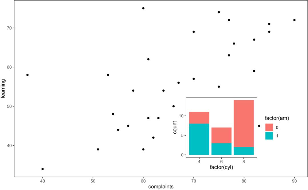
#源代码： R语言统计与绘图library(ggplot2)library(grid) # viewport()函数## 绘制主图&子图## 绘制主图plot1<-ggplot(data = attitude)+geom_point(mapping = aes(x = complaints, y = learning))+theme_bw()+ theme(panel.grid.major=element_line(colour=NA), panel.background = element_rect(fill = "transparent",colour = NA), plot.background = element_rect(fill = "transparent",colour = NA), panel.grid.minor = element_blank())## 绘制子图plot2<-ggplot(mtcars,aes(factor(cyl),fill=factor(am)))+geom_bar()+theme_bw()+ theme(panel.grid.major=element_line(colour=NA), panel.background = element_rect(fill = "transparent",colour = NA), plot.background = element_rect(fill = "transparent",colour = NA), panel.grid.minor = element_blank())## 设置子图的位置和大小subplot1<- viewport(width=0.4,height=0.4,x=0.6,y=0.5)## 绘制子图嵌套plot1print(plot2, vp=subplot1) subplot2<-viewport(width=0.4,height=0.4,x=0.75,y=0.30) # 要再次生成图片哦~plot1print(plot2, vp=subplot2) 

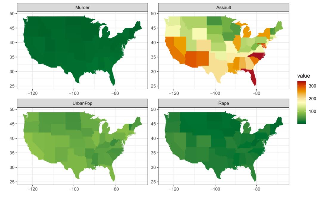
library(ggplot2)library(maps)library(paletteer)crimes <- data.frame(state = tolower(rownames(USArrests)), USArrests)vars <- lapply(names(crimes)[-1], function(j) {data.frame(state = crimes$state, variable = j, value = crimes[[j]])})crimes_long <- do.call("rbind", vars)states_map <- map_data("state")ggplot(crimes_long, aes(map_id = state)) +geom_map(aes(fill = value), map = states_map) +expand_limits(x = states_map$long, y = states_map$lat) +facet_wrap( ~ variable)+paletteer::scale_fill_paletteer_c("grDevices::RdYlGn", direction = -1)+theme_bw()

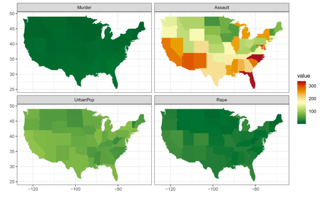
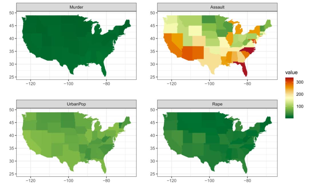
library(ggplot2)library(maps)library(paletteer)crimes <- data.frame(state = tolower(rownames(USArrests)), USArrests)vars <- lapply(names(crimes)[-1], function(j) {data.frame(state = crimes$state, variable = j, value = crimes[[j]])})crimes_long <- do.call("rbind", vars)states_map <- map_data("state")ggplot(crimes_long, aes(map_id = state)) +geom_map(aes(fill = value), map = states_map) +expand_limits(x = states_map$long, y = states_map$lat) +facet_wrap( ~ variable,scales="free")+paletteer::scale_fill_paletteer_c("grDevices::RdYlGn", direction = -1)+theme_bw()

library(ggplot2)library(maps)library(paletteer)crimes <- data.frame(state = tolower(rownames(USArrests)), USArrests)vars <- lapply(names(crimes)[-1], function(j) {data.frame(state = crimes$state, variable = j, value = crimes[[j]])})crimes_long <- do.call("rbind", vars)states_map <- map_data("state")ggplot(crimes_long, aes(map_id = state)) +geom_map(aes(fill = value), map = states_map) +expand_limits(x = states_map$long, y = states_map$lat) +facet_wrap( ~ variable,scales="free")+paletteer::scale_fill_paletteer_c("grDevices::RdYlGn", direction = -1)+theme_bw()+theme(panel.spacing.x = unit(1, "cm"),panel.spacing.y = unit(1, "cm"))

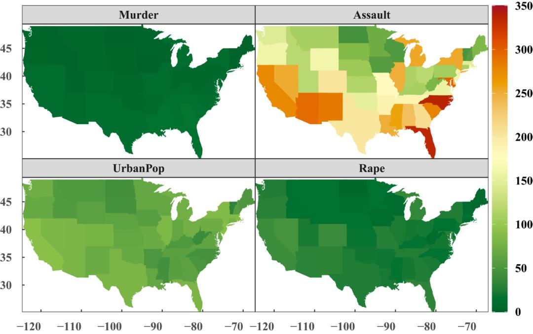
library(ggplot2)library(maps)library(paletteer)crimes <- data.frame(state = tolower(rownames(USArrests)), USArrests)vars <- lapply(names(crimes)[-1], function(j) {data.frame(state = crimes$state, variable = j, value = crimes[[j]])})crimes_long <- do.call("rbind", vars)states_map <- map_data("state")ggplot(crimes_long, aes(map_id = state)) +geom_map(aes(fill = value), map = states_map) +expand_limits(x = states_map$long, y = states_map$lat) +facet_wrap( ~ variable)+paletteer::scale_fill_paletteer_c("grDevices::RdYlGn", direction = -1, breaks = c(0,50,100,150,200,250,300,350),labels = c(0,50,100,150,200,250,300,350),limits = c(0,350))+ theme_bw() + # 去除地图灰色背景 theme(panel.grid.major=element_line(colour=NA), panel.background = element_rect(fill = "transparent",colour = NA), plot.background = element_rect(fill = "transparent",colour = NA), panel.grid.minor = element_blank())+ # 去除地图网格theme(axis.ticks.length=unit(-0.1, "cm"), axis.text.x = element_text(margin=unit(c(0.5,0.5,0.5,0.5), "cm")), axis.text.y = element_text(margin=unit(c(0.5,0.5,0.5,0.5), "cm")) )+ theme(axis.text.x = element_text(angle=0,hjust=1), # 旋转坐标轴label的方向 text = element_text(size = 16, face = "bold", family="serif"),  panel.spacing = unit(0,"lines") )+ #分面间隔设为零scale_y_continuous(expand = c(0,0))+ #这个可以图形去掉与X轴间隙scale_x_continuous(expand = c(0,0))+theme(legend.key.height = grid::unit(2.4, "cm"))

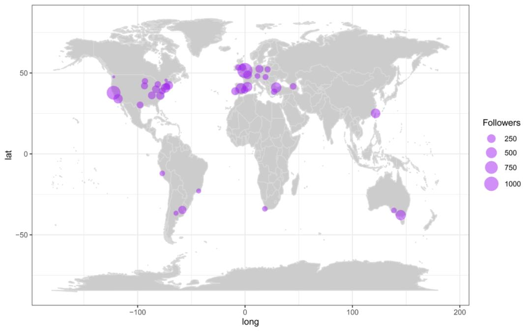
library(readr)library(dplyr)url_csv <- 'https://raw.githubusercontent.com/d4tagirl/R-Ladies-growth-maps/master/rladies.csv'rladies <- read_csv(url(url_csv)) %>% select(-1)library(DT)datatable(rladies, rownames = FALSE,options = list(pageLength = 5))library(ggplot2)library(maps)library(ggthemes)world <- ggplot() +borders("world", colour = "gray85", fill = "gray80") +theme_bw()map <- world +geom_point(aes(x = lon, y = lat, size = followers),data = rladies, colour = 'purple', alpha = .5) + scale_size_continuous(range = c(1, 8), breaks = c(250, 500, 750, 1000)) +labs(size = 'Followers')map

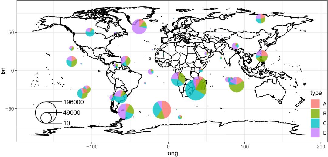
set.seed(123)long <- rnorm(50, sd=100)lat <- rnorm(50, sd=50)d <- data.frame(long=long, lat=lat)d <- with(d, d[abs(long) < 150 & abs(lat) < 70,])n <- nrow(d)d$region <- factor(1:n)d$A <- abs(rnorm(n, sd=1))d$B <- abs(rnorm(n, sd=2))d$C <- abs(rnorm(n, sd=3))d$D <- abs(rnorm(n, sd=4))d[1, 4:7] <- d[1, 4:7] * 3head(d)ggplot() + geom_scatterpie(aes(x=long, y=lat, group=region), data=d,cols=LETTERS[1:4]) + coord_equal()+theme_bw()d$radius <- 6 * abs(rnorm(n))p <- ggplot() + geom_scatterpie(aes(x=long, y=lat, group=region, r=radius), data=d,cols=LETTERS[1:4], color=NA) + coord_equal()p + geom_scatterpie_legend(d$radius, x=-140, y=-70)+theme_bw()world <- map_data('world')p <- ggplot(world, aes(long, lat)) +geom_map(map=world, aes(map_id=region), fill=NA, color="black") +coord_quickmap()p + geom_scatterpie(aes(x=long, y=lat, group=region, r=radius),data=d, cols=LETTERS[1:4], color=NA, alpha=.8) +    geom_scatterpie_legend(d$radius, x=-160, y=-55)+theme_bw()p + geom_scatterpie(aes(x=long, y=lat, group=region, r=radius),data=d, cols=LETTERS[1:4], color=NA, alpha=.8) + geom_scatterpie_legend(d$radius, x=-160, y=-55, n=3, labeller=function(x) 1000*x^2)+theme_bw()

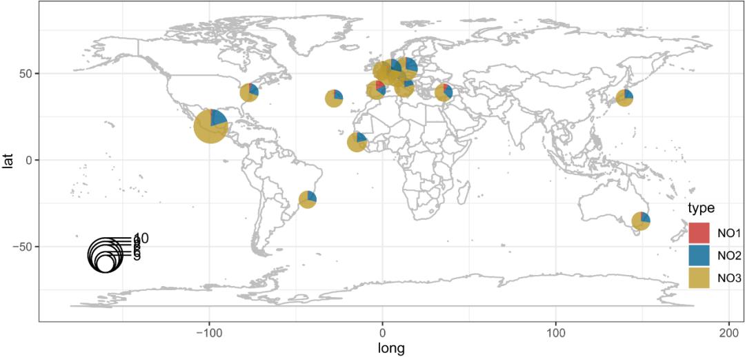
library(ggplot2)library(plyr)library("maptools")library(scatterpie)world_map <-readShapePoly("F:/Rpeng/29/data/World_region.shp")x <- world_map@data xs <- data.frame(x,id=seq(0:250)-1) world_map1 <- fortify(world_map) world_map_data <- join(world_map1, xs, type = "full") mydata<-read.csv("F:/Rpeng/29/data/WorldGDP.csv",header=T,encoding='UTF-8',stringsAsFactors = FALSE) midpos <- function(x) mean(range(x,na.rm=TRUE))centres <- ddply(world_map_data,.(COUNTRY),colwise(midpos,.(long,lat)))mapdata<-merge(centres,mydata,by.x="COUNTRY",by.y="FULLName",all.y=TRUE)mapdata$order<-as.factor(mapdata$order)mapdata$point<-5*mapdata$GDP/max(mapdata$GDP)+5value<-names(mapdata)[8:10]mapdata[1,c("long","lat")]<-c(-77.013222,38.913611) #华盛顿mapdata[2,c("long","lat")]<-c(2.329671,48.871029) #巴黎mapdata[3,c("long","lat")]<-c(-0.124969,51.516434) #伦敦mapdata[4,c("long","lat")]<-c(12.496336,41.91076) #罗马mapdata[5,c("long","lat")]<-c(4.882042,52.372936) #阿姆斯特丹mapdata[6,c("long","lat")]<-c(-3.704783,40.421502) #马德里mapdata[7,c("long","lat")]<-c(139.650947,35.833005) #东京mapdata[8,c("long","lat")]<-c(13.407002,52.527935) #柏林mapdata[9,c("long","lat")]<-c(8.45468,47.440827) #苏黎世mapdata[11,c("long","lat")]<-c(149.116199,-35.315167) #墨尔本mapdata[12,c("long","lat")]<-c(-43.264882,-22.895071) #里约热内卢mapdata[15,c("long","lat")]<-c(-99.129758,19.449516) #墨西哥城 ggplot(world_map_data,aes(x=long, y=lat,group=group)) +geom_polygon(fill="white", color="grey")+ geom_scatterpie(data=mapdata,aes(x=long, y=lat,group=order,r=point),cols=value,color=NA, alpha=.8) + coord_equal()+geom_scatterpie_legend(mapdata$point, x=-160, y=-55)+    scale_fill_wsj()+theme_bw()world <- map_data('world')ggplot(world, aes(long, lat,group=group)) +geom_polygon(fill="white", color="grey")+ geom_scatterpie(data=mapdata,aes(x=long, y=lat,group=order,r=point),cols=value,color=NA, alpha=.8) + coord_equal()+geom_scatterpie_legend(mapdata$point, x=-160, y=-55)+    scale_fill_wsj()+theme_bw()

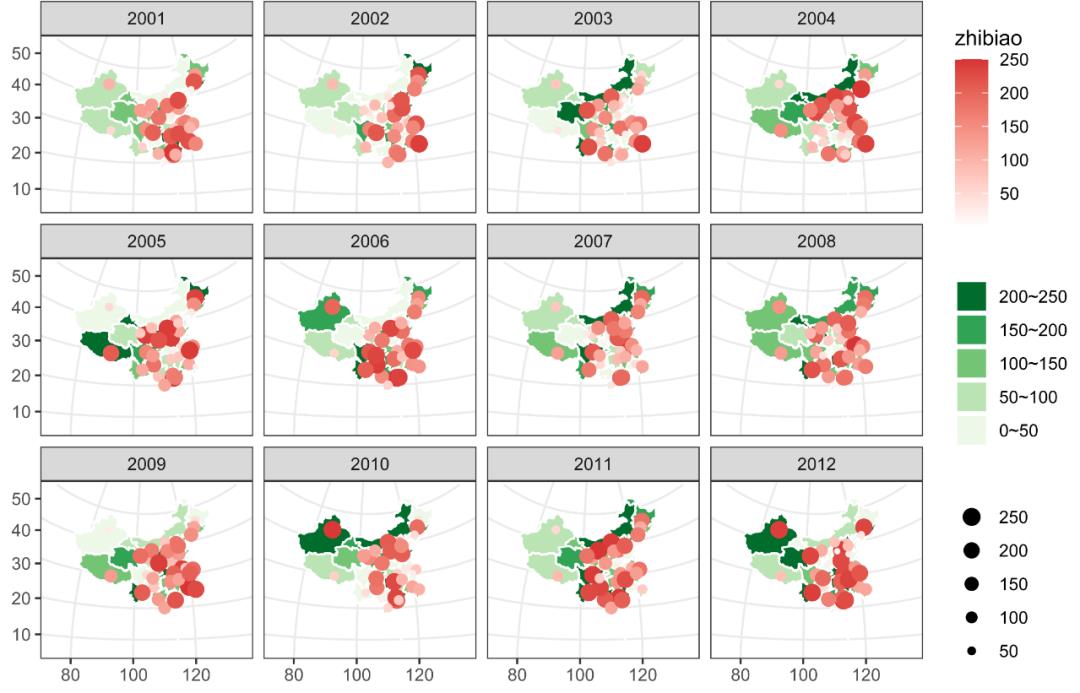
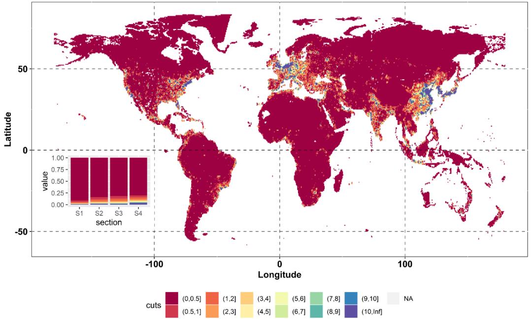
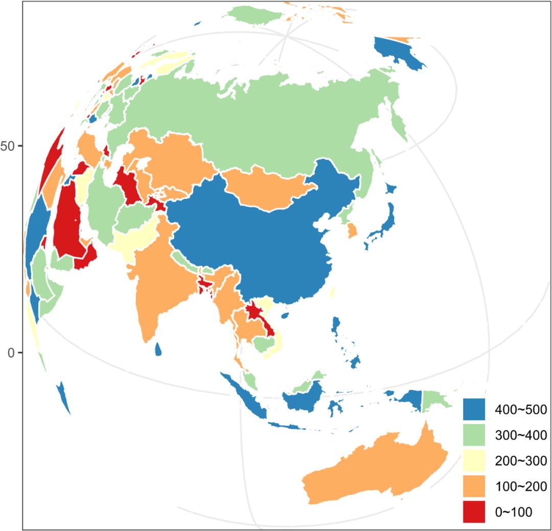
library("ggplot2")library("plyr")library("maptools")library("ggthemes")options(stringsAsFactors=FALSE,warn=FALSE)world_map <-readShapePoly("F:/Rpeng/29/data/World_region.shp")x <- world_map@data xs <- data.frame(x,id=seq(0:250)-1) world_map1 <- fortify(world_map) world_map_data <- join(world_map1, xs, type = "full")mydata <- read.csv("F:/Rpeng/29/data/Region_map.csv") mydata$fam<-cut(mydata$zhibiao1,breaks=c(0,100,200,300,400,500),labels=c('0~100','100~200','200~300','300~400','400~500'),order=TRUE,include.lowest=TRUE)world_data <- join(world_map_data, mydata, type="full")ggplot(world_data, aes(x = long, y = lat, group = group,fill =fam))+geom_polygon(colour="white")+scale_fill_brewer(palette="Spectral")+ coord_map("ortho", orientation = c(30, 110, 0))+guides(fill=guide_legend(reverse=TRUE,title=NULL))+theme_map()+theme_bw()

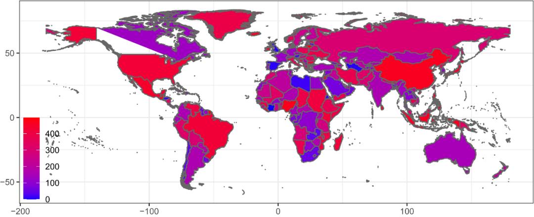
library(ggplot2)library(plyr)library("maptools")#导入并整理世界地图地理信息数据：world_map <-readShapePoly("F:/Rpeng/29/data/World_region.shp")x <- world_map@data #读取行政信息xs <- data.frame(x,id=seq(0:250)-1) #含岛屿共251个形状world_map1 <- fortify(world_map) #转化为数据框world_map_data <- join(world_map1, xs, type = "full") #合并两个数据框#导入指标文件数据并合并成作图数据：mydata <- read.csv("F:/Rpeng/29/data/Region_map.csv") #读取指标数据，csv格式world_data <- join(world_map_data, mydata, type="full") #合并两个数据框ggplot(world_data, aes(x = long, y = lat, group = group,fill = zhibiao1)) + geom_polygon(colour="grey40") +scale_fill_gradient(low="blue",high="red") +theme_bw()+coord_equal()

library(ggplot2)library(plyr)library("maptools")American_map <-readShapePoly("F:/Rpeng/29/data/STATES.SHP") #将地理信息数据导入R环境x <- American_map@data #读取行政信息xs <- data.frame(x,id=seq(0:50)-1) #共51个形状American_map1 <- fortify(American_map) #转化为数据框American_map_data <- join(American_map1, xs, type = "full") #合并两个数据框mydata <- read.csv("F:/Rpeng/29/data/USA_data.csv")#读取业务指标数据，csv格式American_data <- join(American_map_data, mydata, type="full") #合并两个数据框ggplot(American_data, aes(x = long, y = lat, group = group,fill = Sale)) + geom_polygon(colour="grey40") +scale_fill_gradient(low="white",high="steelblue") + #指定渐变填充色，可使用RGB #coord_map("polyconic") + #指定投影方式为polyconic，获得常见视角美国地图，如要获得平面视角地图，此句可省略 theme(panel.grid = element_blank(),panel.background = element_blank(), axis.text = element_blank(),axis.ticks = element_blank(),axis.title = element_blank(),legend.position = c(0.1,0.3))+theme_bw() library(paletteer)ggplot(American_data, aes(x = long, y = lat, group = group,fill = Sale)) + geom_polygon(colour="grey40") +paletteer::scale_fill_paletteer_c("grDevices::RdYlGn", direction = -1)+ theme(panel.grid = element_blank(),panel.background = element_blank(), axis.text = element_blank(),axis.ticks = element_blank(),axis.title = element_blank(),legend.position = c(0.1,0.3))+theme_bw() 

待续............................待续............................待续............................

---

---

只要你点下方【分享】【赞】【在看】

我们就是好朋友，Thanks♪(･ω･)ﾉ