Pytorch Note10 多项式回归

Posted 2021-06-27 Real&Love

Pytorch Note10 多项式回归

• • 多项式回归
  • 定义多项式模型
  • 定义损失函数和优化器
  • 训练模型
  • 模型参数
  • 测试模型

全部笔记的汇总贴：Pytorch Note 快乐星球

多项式回归

什么是多项式回归呢？非常简单，根据上面的线性回归模型

$$\hat{y}=wx+b$$

这里是关于 x 的一个一次多项式，这个模型比较简单，没有办法拟合比较复杂的模型，所以我们可以使用更高次的模型，比如

$$\hat{y}=w_0+w_{1}x+w_2{x}^2+w_3{x}^3+\cdots$$

对于一般的线性回归，由于该函数拟合出来的是一条直线，所以精度欠佳，我们可以考虑多项式回归，也就是提高每个属性的次数，而不再是只使用一次去回归目标函数。原理和之前的线性回归是一样的，只不过这里用的是高次多项式而不是简单的一次线性多项式。首先给出我们想要拟合的方程：

$y=0.9+0.5\times x+3\times x^2+2.4\times x^3$

然后可以设置参数方程：

$y=b+w_1\times x+w_2\times x^2+w_3\times x^3$

我们希望每一个参数都能够学习到和真实参数很接近的结果。下面来看看如何用 PyTorch 实现这个简单的任务。

首先需要预处理数据，也就是需要将数据变成一个矩阵的形式：

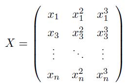
在 PyTorch 里面使用 torch.cat() 函数来实现 Tensor 的拼接：

def make_features(x):
    '''Builds features i.. a matrix with columns [x,x^2,x^3].'''
    x = x.unsqueeze(1)
    return torch.cat([x ** i for i in range(1,4)],1)

对于输入的 n 个数据，我们将其扩展成上面矩阵所示的样子。

然后定义好真实的函数：

W_target = torch.FloatTensor([0.5, 3, 2.4]).unsqueeze(1) # 增加第二维
b_target = torch.FloatTensor([0.9])

def f(x):
    '''Approximated function'''
    return torch.mm(x,W_target) + b_target[0] # x.mm做矩阵乘法

这里的权重已经定义好了，unsqueeze(1)是将原来的 tensor 大小由 3 变成 (3, 1)，torch.mm(x,W_target) 表示做矩阵乘法，f (x) 就是每次输入一个 x 得到一个 y 的真实函数。

f_res = 'y = {:.2f} + {:.2f} * x + {:.2f} * x^2 + {:.2f} * x^3'.format(b_target[0],W_target[0][0],W_target[1][0],W_target[2][0])
print(f_res)

y = 0.90 + 0.50 * x + 3.00 * x^2 + 2.40 * x^3

在进行训练的时候我们需要采样一些点，可以随机生成一些数来得到每次的训练集：

def get_batch(batch_size = 30):
    '''Builds a batch i.e. (x,f(x)) pair'''
    random = torch.randn(batch_size)
    x = make_features(random)
    y = f(x)
    if torch.cuda.is_available():
        return Variable(x).cuda(),Variable(y).cuda()
    else:
        return Variable(x),Variable(y)

定义多项式模型

# Define model
class poly_model(nn.Module):
    def __init__(self):
        super(poly_model, self).__init__()
        self.poly = nn.Linear(3,1)
        
    def forward(self, x):
        out = self.poly(x)
        return out

if torch.cuda.is_available():
    model = poly_model().cuda()
else:
    model = poly_model()

定义损失函数和优化器

criterion  =  nn.MSELoss()
optimizer  =  optim.SGD(model.parameters(),  lr=1e-3)

训练模型

epoch = 0
while True:
    # Get data
    batch_x, batch_y = get_batch()
    # Forward pass
    output = model(batch_x)
    loss = criterion(output, batch_y)
    print_loss = loss.data
    # Reset gradients
    optimizer.zero_grad()
    # Backward pass
    loss.backward()
    # update parameters
    optimizer.step()
    epoch += 1
    if epoch % 100 == 0:
        print('epoch : {}  loss : {}'.format(epoch,print_loss))
    if print_loss < 1e-3:
        break

epoch : 100 loss : 3.394636631011963
epoch : 200 loss : 6.6117262840271
epoch : 300 loss : 0.3985896408557892
epoch : 400 loss : 0.1499343365430832
epoch : 500 loss : 0.0376853384077549
epoch : 600 loss : 0.03172992169857025
epoch : 700 loss : 0.03209806606173515
epoch : 800 loss : 0.045599423348903656
epoch : 900 loss : 0.020373135805130005
epoch : 1000 loss : 0.018576379865407944
epoch : 1100 loss : 0.01291999127715826
epoch : 1200 loss : 0.012883610092103481
epoch : 1300 loss : 0.008911225013434887
epoch : 1400 loss : 0.006300895940512419
epoch : 1500 loss : 0.006056365557014942
epoch : 1600 loss : 0.0041351644322276115
epoch : 1700 loss : 0.003991010598838329
epoch : 1800 loss : 0.002544376067817211
epoch : 1900 loss : 0.00221385364420712
epoch : 2000 loss : 0.0016465323278680444

这里我们希望模型能够不断地优化，直到实现我们设立的条件，取出的 32 个点的均方误差能够小于 0.001

模型参数

model.state_dict().items()

odict_items([(‘poly.weight’, tensor([[0.4918, 2.9820, 2.4022]], device=‘cuda:0’)), (‘poly.bias’, tensor([0.9459], device=‘cuda:0’))])

print('weight : ',model.state_dict()['poly.weight'])
print('bias : ',model.state_dict()['poly.bias'])

weight : tensor([[0.4918, 2.9820, 2.4022]], device=‘cuda:0’)
bias : tensor([0.9459], device=‘cuda:0’)

w = torch.ones_like(W_target)
for i in range(3):
    w[i] = model.state_dict()['poly.weight'][0][i].cpu()
w = w.numpy()

b = model.state_dict()['poly.bias']
b = b[0].cpu().numpy()

测试模型

得到(-1,1)的点，进行一个测试

x = np.arange(-1,1,0.1)
x = torch.from_numpy(x).float()
x = make_features(x).squeeze()

plt.plot(x[:,0],f(x),'ro',label = 'real')

a = np.arange(-1,1,0.1)
plt.plot(a,b + w[0]*a + w[1]*a*a+ w[2]*a*a*a, label = 'fitting')
plt.legend()

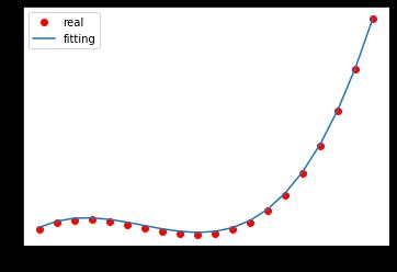
将真实函数的数据点和拟合的多项式画在同一张图上，可以得到上图

下一章传送门：Note11 Logistic 回归模型