卷积神经网络参数解析

Posted 2023-03-27

参考技术A （1）现象：

        （1-1）一次性将batch数量个样本feed神经网络，进行前向传播；然后再进行权重的调整，这样的一整个过程叫做一个回合（epoch），也即一个batch大小样本的全过程就是一次迭代。

        （1-2）将训练数据分块，做成批(batch training)训练可以将多个训练数据元的loss function求和，使用梯度下降法，最小化 求和后的loss function ，进而对神经网络的参数进行优化更新

（2）一次迭代：包括前向传播计算输出向量、输出向量与label的loss计算和后向传播求loss对权重向量 w 导数（梯度下降法计算），并实现权重向量 w 的更新。

（3）优点：

        （a）对梯度向量（代价函数对权值向量 w 的导数）的精确估计，保证以最快的速度下降到局部极小值的收敛性；一个batch一次梯度下降；

        （b）学习过程的并行运行；

        （c）更加接近随机梯度下降的算法效果；

        （d）Batch Normalization 使用同批次的统计平均和偏差对数据进行正则化，加速训练，有时可提高正确率 [7]

（4）现实工程问题：存在计算机存储问题，一次加载的batch大小受到内存的影响；

（5）batch参数选择：

        （5-1）从收敛速度的角度来说，小批量的样本集合是最优的，也就是我们所说的mini-batch，这时的batch size往往从几十到几百不等，但一般不会超过几千

        （5-2）GPU对2的幂次的batch可以发挥更佳的性能，因此设置成16、32、64、128...时往往要比设置为整10、整100的倍数时表现更优

    （6）4种加速批梯度下降的方法 [8] ：

        （6-1）使用动量－使用权重的 速度 而非 位置 来改变权重。

        （6-2）针对不同权重参数使用不同学习率。

        （6-3）RMSProp－这是Prop 的均方根 ( Mean Square ) 改进形式，Rprop 仅仅使用梯度的符号，RMSProp 是其针对 Mini-batches 的平均化版本

        （6-4）利用曲率信息的最优化方法。

（1）定义：运用梯度下降算法优化loss成本函数时，权重向量的更新规则中，在梯度项前会乘以一个系数，这个系数就叫学习速率η

（2）效果：

        （2-1）学习率η越小，每次迭代权值向量变化小，学习速度慢，轨迹在权值空间中较光滑，收敛慢；

        （2-2）学习率η越大，每次迭代权值向量变化大，学习速度快，但是有可能使变化处于震荡中，无法收敛；

    （3）处理方法：

        （3-1）既要加快学习速度又要保持稳定的方法修改delta法则，即添加动量项。

    （4）选择经验：

        （4-1）基于经验的手动调整。 通过尝试不同的固定学习率，如0.1, 0.01, 0.001等，观察迭代次数和loss的变化关系，找到loss下降最快关系对应的学习率。

        （4-2）基于策略的调整。

                （4-2-1）fixed 、exponential、polynomial

                （4-2-2）自适应动态调整。adadelta、adagrad、ftrl、momentum、rmsprop、sgd

    （5）学习率η的调整：学习速率在学习过程中实现自适应调整（一般是衰减）

        （5-1）非自适应学习速率可能不是最佳的。

        （5-2）动量是一种自适应学习速率方法的参数，允许沿浅方向使用较高的速度，同时沿陡峭方向降低速度前进

        （5-3）降低学习速率是必要的，因为在训练过程中，较高学习速率很可能陷入局部最小值。

参考文献：

[1]  Simon Haykin. 神经网络与机器学习[M]. 机械工业出版社, 2011.

[2]   训练神经网络时如何确定batch的大小？

[3]   学习笔记：Batch Size 对深度神经网络预言能力的影响  

[4]   机器学习算法中如何选取超参数：学习速率、正则项系数、minibatch size.  http://blog.csdn.net/u012162613/article/details/44265967

[5]   深度学习如何设置学习率 . http://blog.csdn.net/mao_feng/article/details/52902666

[6]   调整学习速率以优化神经网络训练. https://zhuanlan.zhihu.com/p/28893986

[7]   机器学习中用来防止过拟合的方法有哪些？

[8]   Neural Networks for Machine Learning by Geoffrey Hinton .

[9]   如何确定卷积神经网络的卷积核大小、卷积层数、每层map个数

[10]   卷积神经网络的卷积核大小、卷积层数、每层map个数都是如何确定下来的呢？

YOLOv5-6.0 源码解析 —— 卷积神经单元

YOLOv5 源码中，模型是依靠 yaml 文件建立的。而 yaml 文件中涉及到的卷积神经网络单元都是在 models 文件夹中的 common.py 声明的，所以自行设计网络结构之前有必要详解这个文件。这个文件很细节，就算不学 YOLOv5 也建议 copy 收藏

通用参数

c1	c2	c_	k	s	p	g	act	shortcut
输入信号 通道	卷积产生 通道	隐藏层 通道	卷积核 尺寸	卷积 步长	边界 填充	卷积 组数	激活 函数	残差 连接

autopad

def autopad(k, p=None):  # kernel, padding
    # Pad to 'same'
    if p is None:
        p = k // 2 if isinstance(k, int) else [x // 2 for x in k]  # auto-pad
    return p

• 如果有既定的 p 则直接 return
• 如果无设定的 p，则 return 使图像在卷积操作后尺寸不变的 p：

1. 如果 k 是 5，则 p = 5 // 2 = 2
2. 如果 k 是 (5, 5)，则 p = (5, 5) // 2 = (2, 2)

Conv

标准卷积单元，记为 CBS

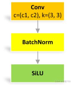
class Conv(nn.Module):
    # Standard convolution
    def __init__(self, c1, c2, k=1, s=1, p=None, g=1, act=True):  # ch_in, ch_out, kernel, stride, padding, groups
        super().__init__()
        self.conv = nn.Conv2d(c1, c2, k, s, autopad(k, p), groups=g, bias=False)
        self.bn = nn.BatchNorm2d(c2)
        self.act = nn.SiLU() if act is True else (act if isinstance(act, nn.Module) else nn.Identity())

    def forward(self, x):
        return self.act(self.bn(self.conv(x)))

    def forward_fuse(self, x):
        return self.act(self.conv(x))

DWConv

深度可分离卷积，继承自 Conv

不同点：卷积组数是 c1 和 c2 的最大公约数

class DWConv(Conv):
    # Depth-wise convolution class
    def __init__(self, c1, c2, k=1, s=1, act=True):  # ch_in, ch_out, kernel, stride, padding, groups
        super().__init__(c1, c2, k, s, g=math.gcd(c1, c2), act=act)

TransformerLayer

单头注意力：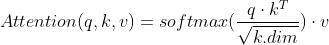

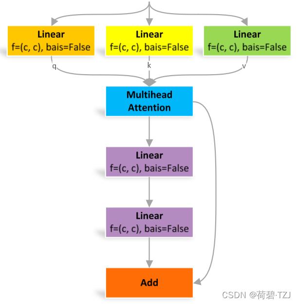
多头注意力：q, k, v 均是长度 c 的向量，单头注意力也是长度 c 的向量，n 的单头注意力拼接后得到长度 nc 的行向量。经过线性层运算后再得到长度 c 的向量 

class TransformerLayer(nn.Module):
    # Transformer layer https://arxiv.org/abs/2010.11929 (LayerNorm layers removed for better performance)
    def __init__(self, c, num_heads):
        super().__init__()
        self.q = nn.Linear(c, c, bias=False)
        self.k = nn.Linear(c, c, bias=False)
        self.v = nn.Linear(c, c, bias=False)
        self.ma = nn.MultiheadAttention(embed_dim=c, num_heads=num_heads)
        self.fc1 = nn.Linear(c, c, bias=False)
        self.fc2 = nn.Linear(c, c, bias=False)

    def forward(self, x):
        x = self.ma(self.q(x), self.k(x), self.v(x))[0] + x
        x = self.fc2(self.fc1(x)) + x
        return x

TransformerBlock

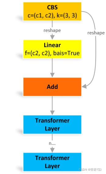
reshape：原图像是 [batch, channel, height, width]，变换成 [height × width, batch, channel]

这个结构原本是用于自然语言处理的，但是据说用在图像处理有奇效就引入了。reshape 操作其实就是把图像中各个像素点看作一个单词，其对应通道的信息连在一起就是词向量，用自然语言处理的方法处理之后，再变回原来的图像结构

class TransformerBlock(nn.Module):
    # Vision Transformer https://arxiv.org/abs/2010.11929
    def __init__(self, c1, c2, num_heads, num_layers):
        super().__init__()
        self.conv = None
        if c1 != c2:
            self.conv = Conv(c1, c2)
        self.linear = nn.Linear(c2, c2)  # learnable position embedding
        self.tr = nn.Sequential(*[TransformerLayer(c2, num_heads) for _ in range(num_layers)])
        self.c2 = c2

    def forward(self, x):
        if self.conv is not None:
            x = self.conv(x)
        b, _, w, h = x.shape
        p = x.flatten(2).unsqueeze(0).transpose(0, 3).squeeze(3)
        return self.tr(p + self.linear(p)).unsqueeze(3).transpose(0, 3).reshape(b, self.c2, w, h)

Bottleneck

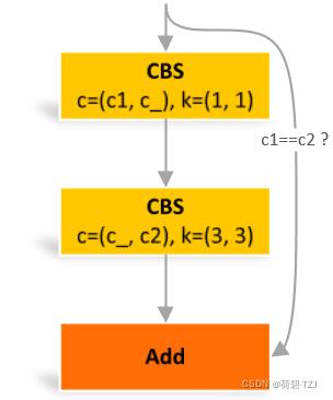
瓶颈卷积，其特点在于隐藏层的通道数 c_ 小于 c2

class Bottleneck(nn.Module):
    # Standard bottleneck
    def __init__(self, c1, c2, shortcut=True, g=1, e=0.5):  # ch_in, ch_out, shortcut, groups, expansion
        super().__init__()
        c_ = int(c2 * e)  # hidden channels
        self.cv1 = Conv(c1, c_, 1, 1)
        self.cv2 = Conv(c_, c2, 3, 1, g=g)
        self.add = shortcut and c1 == c2

    def forward(self, x):
        return x + self.cv2(self.cv1(x)) if self.add else self.cv2(self.cv1(x))

BottleneckCSP

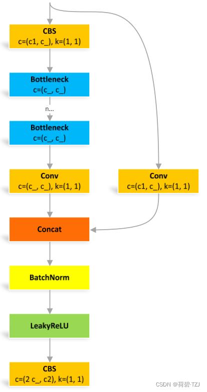
class BottleneckCSP(nn.Module):
    # CSP Bottleneck https://github.com/WongKinYiu/CrossStagePartialNetworks
    def __init__(self, c1, c2, n=1, shortcut=True, g=1, e=0.5):  # ch_in, ch_out, number, shortcut, groups, expansion
        super().__init__()
        c_ = int(c2 * e)  # hidden channels
        self.cv1 = Conv(c1, c_, 1, 1)
        self.cv2 = nn.Conv2d(c1, c_, 1, 1, bias=False)
        self.cv3 = nn.Conv2d(c_, c_, 1, 1, bias=False)
        self.cv4 = Conv(2 * c_, c2, 1, 1)
        self.bn = nn.BatchNorm2d(2 * c_)  # applied to cat(cv2, cv3)
        self.act = nn.LeakyReLU(0.1, inplace=True)
        self.m = nn.Sequential(*[Bottleneck(c_, c_, shortcut, g, e=1.0) for _ in range(n)])

    def forward(self, x):
        y1 = self.cv3(self.m(self.cv1(x)))
        y2 = self.cv2(x)
        return self.cv4(self.act(self.bn(torch.cat((y1, y2), dim=1))))

C3

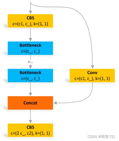
与 BottleneckCSP 类似，但少了 1 个 Conv、1 个 BN、1 个 Act，运算量更少

class C3(nn.Module):
    # CSP Bottleneck with 3 convolutions
    def __init__(self, c1, c2, n=1, shortcut=True, g=1, e=0.5):  # ch_in, ch_out, number, shortcut, groups, expansion
        super().__init__()
        c_ = int(c2 * e)  # hidden channels
        self.cv1 = Conv(c1, c_, 1, 1)
        self.cv2 = Conv(c1, c_, 1, 1)
        self.cv3 = Conv(2 * c_, c2, 1)  # act=FReLU(c2)
        self.m = nn.Sequential(*[Bottleneck(c_, c_, shortcut, g, e=1.0) for _ in range(n)])
        # self.m = nn.Sequential(*[CrossConv(c_, c_, 3, 1, g, 1.0, shortcut) for _ in range(n)])

    def forward(self, x):
        return self.cv3(torch.cat((self.m(self.cv1(x)), self.cv2(x)), dim=1))

C3TR

继承自 C3，n 个 Bottleneck 更换为 1 个 TransformerBlock

class C3TR(C3):
    # C3 module with TransformerBlock()
    def __init__(self, c1, c2, n=1, shortcut=True, g=1, e=0.5):
        super().__init__(c1, c2, n, shortcut, g, e)
        c_ = int(c2 * e)
        self.m = TransformerBlock(c_, c_, 4, n)

C3SPP

继承自 C3，n 个 Bottleneck 更换为 1 个 SPP

class C3SPP(C3):
    # C3 module with SPP()
    def __init__(self, c1, c2, k=(5, 9, 13), n=1, shortcut=True, g=1, e=0.5):
        super().__init__(c1, c2, n, shortcut, g, e)
        c_ = int(c2 * e)
        self.m = SPP(c_, c_, k)

C3Ghost

继承自 C3，Bottleneck 更换为 GhostBottleneck

class C3Ghost(C3):
    # C3 module with GhostBottleneck()
    def __init__(self, c1, c2, n=1, shortcut=True, g=1, e=0.5):
        super().__init__(c1, c2, n, shortcut, g, e)
        c_ = int(c2 * e)  # hidden channels
        self.m = nn.Sequential(*[GhostBottleneck(c_, c_) for _ in range(n)])

GhostConv

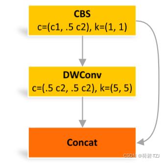
class GhostConv(nn.Module):
    # Ghost Convolution https://github.com/huawei-noah/ghostnet
    def __init__(self, c1, c2, k=1, s=1, g=1, act=True):  # ch_in, ch_out, kernel, stride, groups
        super().__init__()
        c_ = c2 // 2  # hidden channels
        self.cv1 = Conv(c1, c_, k, s, None, g, act)
        self.cv2 = Conv(c_, c_, 5, 1, None, c_, act)

    def forward(self, x):
        y = self.cv1(x)
        return torch.cat([y, self.cv2(y)], 1)

GhostBottleneck

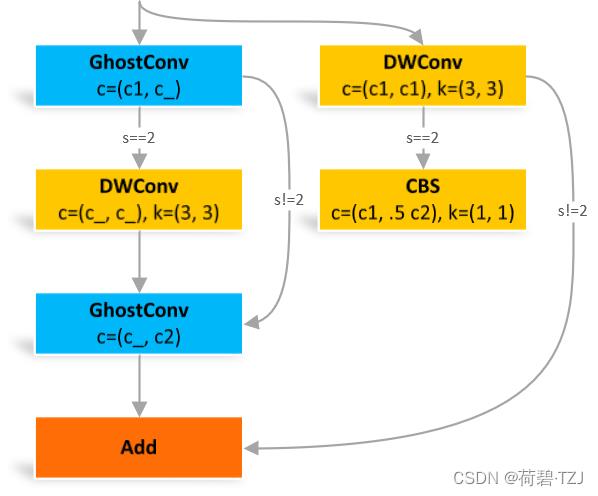
这个结构受步长 s 的影响较大，s = 2 时多了两个卷积 

class GhostBottleneck(nn.Module):
    # Ghost Bottleneck https://github.com/huawei-noah/ghostnet
    def __init__(self, c1, c2, k=3, s=1):  # ch_in, ch_out, kernel, stride
        super().__init__()
        c_ = c2 // 2
        self.conv = nn.Sequential(GhostConv(c1, c_, 1, 1),  # pw
                                  DWConv(c_, c_, k, s, act=False) if s == 2 else nn.Identity(),  # dw
                                  GhostConv(c_, c2, 1, 1, act=False))  # pw-linear
        self.shortcut = nn.Sequential(DWConv(c1, c1, k, s, act=False),
                                      Conv(c1, c2, 1, 1, act=False)) if s == 2 else nn.Identity()

    def forward(self, x):
        return self.conv(x) + self.shortcut(x)

SPP

空间金字塔池化

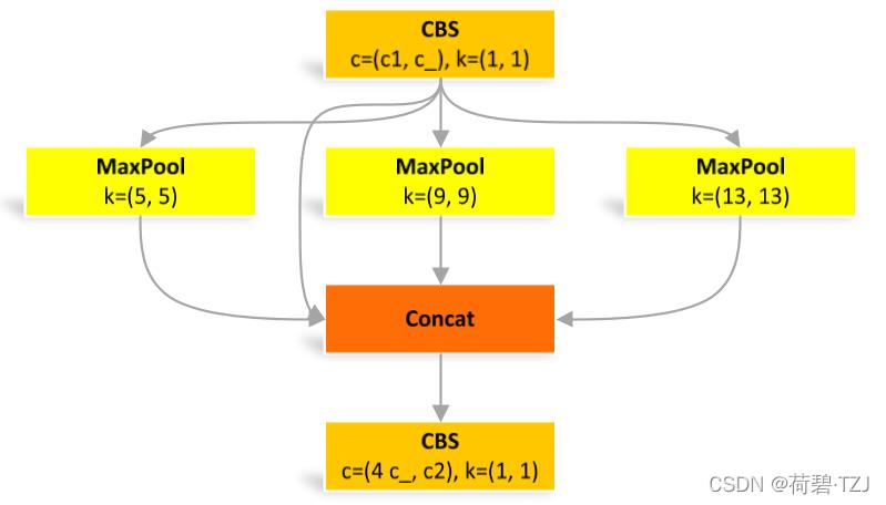
class SPP(nn.Module):
    # Spatial Pyramid Pooling (SPP) layer https://arxiv.org/abs/1406.4729
    def __init__(self, c1, c2, k=(5, 9, 13)):
        super().__init__()
        c_ = c1 // 2  # hidden channels
        self.cv1 = Conv(c1, c_, 1, 1)
        self.cv2 = Conv(c_ * (len(k) + 1), c2, 1, 1)
        self.m = nn.ModuleList([nn.MaxPool2d(kernel_size=x, stride=1, padding=x // 2) for x in k])

    def forward(self, x):
        x = self.cv1(x)
        with warnings.catch_warnings():
            warnings.simplefilter('ignore')  # suppress torch 1.9.0 max_pool2d() warning
            return self.cv2(torch.cat([x] + [m(x) for m in self.m], 1))

SPPF

快速版的空间金字塔池化

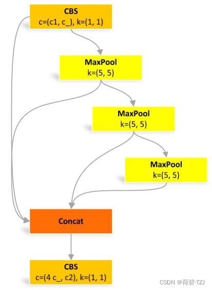
池化尺寸等价于：5、9、13，和原来一样

但是运算量从原来的 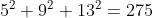 减少到了 

class SPPF(nn.Module):
    # Spatial Pyramid Pooling - Fast (SPPF) layer for YOLOv5 by Glenn Jocher
    def __init__(self, c1, c2, k=5):  # equivalent to SPP(k=(5, 9, 13))
        super().__init__()
        c_ = c1 // 2  # hidden channels
        self.cv1 = Conv(c1, c_, 1, 1)
        self.cv2 = Conv(c_ * 4, c2, 1, 1)
        self.m = nn.MaxPool2d(kernel_size=k, stride=1, padding=k // 2)

    def forward(self, x):
        x = self.cv1(x)
        with warnings.catch_warnings():
            warnings.simplefilter('ignore')  # suppress torch 1.9.0 max_pool2d() warning
            y1 = self.m(x)
            y2 = self.m(y1)
            return self.cv2(torch.cat([x, y1, y2, self.m(y2)], 1))

Focus

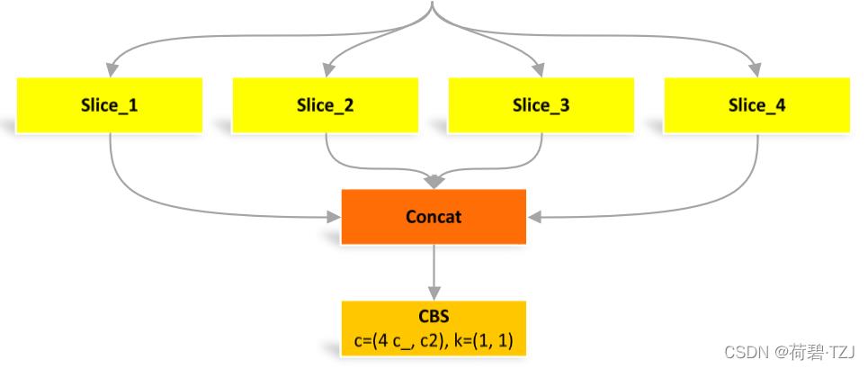
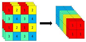
 四个 Slice 是由图像在像素位置上分割出来的

class Focus(nn.Module):
    # Focus wh information into c-space
    def __init__(self, c1, c2, k=1, s=1, p=None, g=1, act=True):  # ch_in, ch_out, kernel, stride, padding, groups
        super().__init__()
        self.conv = Conv(c1 * 4, c2, k, s, p, g, act)
        # self.contract = Contract(gain=2)

    def forward(self, x):  # x(b,c,w,h) -> y(b,4c,w/2,h/2)
        return self.conv(torch.cat([x[..., ::2, ::2], x[..., 1::2, ::2], x[..., ::2, 1::2], x[..., 1::2, 1::2]], 1))
        # return self.conv(self.contract(x))

Contrast

当 gain = 2 的时候，(64, 80, 80) 的图像 -> (256, 40, 40) 的图像。其操作类似 Focus，但更灵活，相比之下少了一个卷积

class Contract(nn.Module):
    # Contract width-height into channels, i.e. x(1,64,80,80) to x(1,256,40,40)
    def __init__(self, gain=2):
        super().__init__()
        self.gain = gain

    def forward(self, x):
        b, c, h, w = x.size()  # assert (h / s == 0) and (W / s == 0), 'Indivisible gain'
        s = self.gain
        x = x.view(b, c, h // s, s, w // s, s)  # x(1,64,40,2,40,2)
        x = x.permute(0, 3, 5, 1, 2, 4).contiguous()  # x(1,2,2,64,40,40)
        return x.view(b, c * s * s, h // s, w // s)  # x(1,256,40,40)

Expand

当 gain = 2 的时候，(1,64,80,80) 的图像 -> (1,16,160,160) 的图像。是 Contrast 的逆操作

class Expand(nn.Module):
    # Expand channels into width-height, i.e. x(1,64,80,80) to x(1,16,160,160)
    def __init__(self, gain=2):
        super().__init__()
        self.gain = gain

    def forward(self, x):
        b, c, h, w = x.size()  # assert C / s ** 2 == 0, 'Indivisible gain'
        s = self.gain
        x = x.view(b, s, s, c // s ** 2, h, w)  # x(1,2,2,16,80,80)
        x = x.permute(0, 3, 4, 1, 5, 2).contiguous()  # x(1,16,80,2,80,2)
        return x.view(b, c // s ** 2, h * s, w * s)  # x(1,16,160,160)

Concat

当 dimension = 1 时，将多张相同尺寸的图像在通道维度上拼接 (通道数可不同)

class Concat(nn.Module):
    # Concatenate a list of tensors along dimension
    def __init__(self, dimension=1):
        super().__init__()
        self.d = dimension

    def forward(self, x):
        return torch.cat(x, self.d)