Matlab数字图像处理学习记录——表示与描述

Posted 2021-05-12 康娜喵

表示与描述

• 零.前言
• 一.背景知识
• • 1.1 单元数组与结构
  • • 1.1.1 单元数组
    • 1.1.2 结构
  • 1.2 一些基本的M函数
• 二.表示
• • 2.1 链码
  • 2.2 使用最小周长多边形的多边形近似
  • 2.3 标记
  • 2.4 边界片断
  • 2.5 骨骼
• 三.边界描绘子
• • 3.1 一些简单的描绘子
  • 3.2 形状数
  • 3.3 傅里叶描绘子
  • 3.4 统计矩
• 四.区域描绘子
• • 4.1 regionprops函数
  • 4.2 纹理
  • • 4.2.1 统计方法
  • 4.2.2 纹理的频谱度量
  • 4.3 不变矩
• 五.主分量描述

零.前言

当我们对一个图像分割为区域后，一般会对分割好的区域进行表示与描述，以便使“自然状态的”像素适合计算机处理。而对于区域有一个基本的划分，为：外部特征(区域的边界)或内部特征(组成区域的像素)两种方式来表示区域。然后下一个任务则是在选择表示的方案的基础上描述区域。比如用图像的边界来表示区域，而边界可以用边界长度、凹面形状数目、凸包等特征来描述。
不过无论选择什么特征，被选做描绘子的特征因该尽量对区域大小、平移、旋转这些变化不敏感。这章描绘子满足一个或多个这样的属性。

一.背景知识

区域是一个连接的分量，而区域的边界则是区域像素的集合，这些像素有一个或多个不存在区域内的相邻像素。不在边界或区域上的点用0来表示，称为背景点。最初使用的是二值图像，通常用1表示边界点，0表示背景。本章后面则会将其扩充到灰度级值或多谱值。
根据上面的定义，可以在得出区域的一些结论：边界是一组相连的点。若边界上的点形成一个顺时针或逆时针序列，则称边界上的点为有序的。若边界上的每个店恰好有两个值均为1的相邻像素点，而且这些像素点不是4邻接的，则称边界是最低限度连接的。内部点定义为区域内擦除边界外的任意位置上的点。
后面的内容会对不同类型的数据进行处理，所以会重新介绍一些基本概念与函数。

1.1 单元数组与结构

1.1.1 单元数组

单元数组可以将各种类型的对象组合在同一个变量名下的方法。比如将512×512的uint8图像f、188×2的二维坐标序列b、包含两个字符名称的单元数组char_arry = {‘area’， ‘centroid’}组合在同一个变量C中的语法为：
C = {f, b, char_array}
若要显示其元素内容，可以：C{3}或celldisp(C{3})。
若使用圆括号，则可以获得变量的描述：

f = zeros(512, 512);
b = ones(188, 2);
char_array = {'area', 'cemtroid'};
C = {f, b, char_array};

C{3}
%%
ans =
  1×2 cell 数组
    {'area'}    {'cemtroid'}
%%

celldisp(C{3})
%%
ans{1} =
area
ans{2} =
cemtroid
%%

C(3)
%%
ans =
  1×1 cell 数组
    {1×2 cell}
%%

1.1.2 结构

结构就是C语言的结构体。结构元素是通过域的名称进行访问的。
假设定义函数：

function s = image_stats(f)
s.dim = size(f);
s.AI = mean2(f);
s.AIrows = mean(f, 2);
s.AIcols = mean(f, 1);

然后我们调用该函数并显示返回的值：

f = imread("./example.tif");
a = image_stats(f);
display(a);
%%
a = 
  包含以下字段的 struct:
       dim: [486 486]
        AI: 0.2805
    AIrows: [486×1 double]
    AIcols: [1×486 double]
%%
size(a)
%%
ans =
     1     1
%%

可以看出结构本身是一个标量。而且使用结构并不会对代码造成更复杂的逻辑，相反可以让输出的数据组织更加清晰，所以这就是面向对象的好处吧。
当然结构也是可以构成数组，且被引用的。这里就不做演示。

1.2 一些基本的M函数

函数B = boundaries(f, conn, dir)可以跟踪f中的对象的外部边界，得到边界的序列。f是默认的二值图像，背景像素为0. conn是输出边界的期望连接方式；其值为4或8连接。参数dir是边界被跟踪的方向，其值为cw和ccw分别代表顺逆时针。这两个参数默认为：8和cw。
假设我们要找对象的唯一最长边界，那么可以：

f = imread('abcd.tif');
gray_f = mat2gray(f);
f = im2bw(gray_f, 0.6);
B = boundaries(f);
d = cellfun('length', B);
[max_d, k] = max(d);
v = B{k(1)}
%%
v =

   152    38
   151    39
   150    39
   149    39
   148    39
…………
   152    38
%%

这样可以得到边界的坐标。
而B刚好包含了四个字母的边界：

%%
B =
  4×1 cell 数组
    {124×2 double}
    {136×2 double}
    {115×2 double}
    {115×2 double}
%%

b8 = bpimd2eoght(b)和b4 = bound2four(b)
输入的b是多行二列的矩阵，每行包含一个边界的像素坐标，且要求这些坐标是闭合的。两个函数会从b中分别保留8连接和4连接的边界。
g = bound2im(b, M, N, x0, y0)生成-幅二值图像g，该图像的大小为M ×N，边界点为1，背景值为0。参数x0和y0决定图像中b的最小x和y坐标位置。边界b必须是坐标的一个大小为np×2(或2×np）的数组，其中,像前面提到的那样，np是点的数目。若x0和y0被省略，则在M×N数组中边界会被近似中心化。若M和N被省略，则图像的水平和垂直尺度就等于边界b的长度和宽度。若函数boundaries发现多个边界，则可以使用函数bound2im，通过连接单元数组B的元素，获得对应的所有坐标:b = cat(1, B{ : })
比如这样：

f = imread('abcd.tif');
subplot(1,2,1);
imshow(f)
[m, n] = size(f);
gray_f = mat2gray(f);
f = im2bw(gray_f, 0.6);
B = boundaries(f);
b = cat(1, B{:});
g = bound2im(b);
subplot(1,2,2);
imshow(g);

二.表示

2.1 链码

链码通过一个指定长度与方向的直线段的连接序列来表示一条边界。每条线段的方向通过编号方案加以编码，得到Freeman编码。就是规定方向，方便搜索。

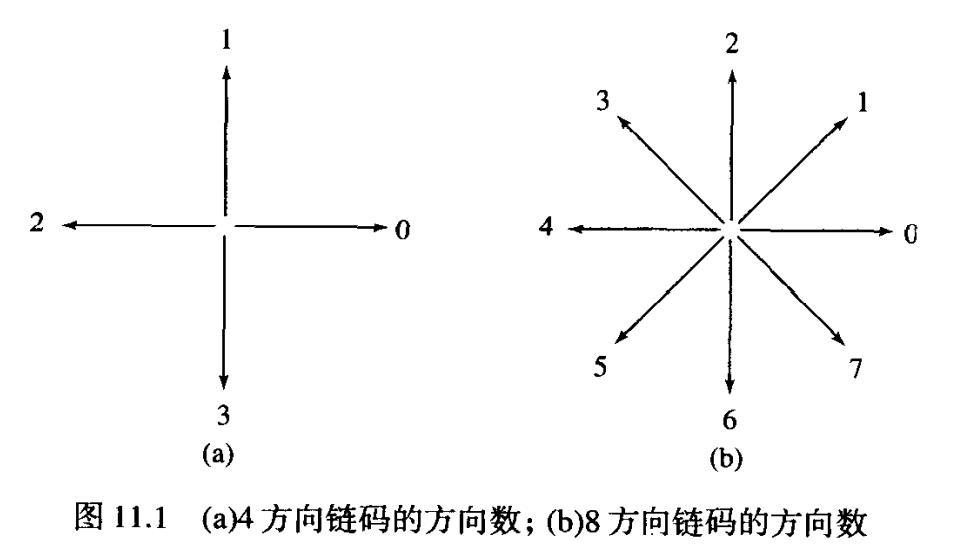
一条边界的链码取决于起点。然而，代码可以通过将起点处理为方向数的循环序列和重新定义起点的方法进行归一化，因此，产生的数字序列形成一个最小幅值的整数。可以通过使用链码的一阶差分来代替链码本身的方法对旋转进行归一化。这种差分可通过计算分隔链码的两个相邻像素的方向变化(图11.1中的逆时针方向)次数来获得。例如，4方向链码10103322的一阶差分为3133030。若我们将链码当做一个循环序列对待，则差分的第一元素可以通过使用链码的第一个和最后一个元素的转换加以计算。这里，结果是33133030。关于任意旋转角度的归一化，可以通过确定带有某些主要特性的边界获得。
用函数c = fchcode(b, conn, dir)
其中：

1. c.fcc 为Freeman链码(1×np)
2. c.diff 为 c.fcc的一节差分(1×np)
3. c.mm 为 最小幅度的整数(1×np)
4. c.diffmm 为代码 c.mm的一阶差分(1×np)
5. c.x0y0 为代码开始处的坐标(1×2)

参数conn是代码连接方式。dir是方向，same或reverse是分别与b同向与反向。默认为8连接同向。
例如:

f = imread('circular.tif');
B = boundaries(f);
d = cellfun('length', B);
[max_d, k] = max(d);
b = B{1};
[m n] = size(f);
g = bound2im(b, m, n, min(b(:, 1)), min(b(:, 2)));
imshow(g2);
[s, su] = bsubsamp(b, 40);
g2 = bound2im(s, m, n, min(s(:, 1)), min(s(:, 2)));
cn = connectpoly(s(:, 1), s(:, 2));
g3 = bound2im(cn, m, n, min(cn(:, 1)), min(cn(:, 2)));
subplot(2,2,1);
imshow(f);
subplot(2,2,2);
imshow(g);
subplot(2,2,3);
imshow(g2);
subplot(2,2,4);
imshow(g3);

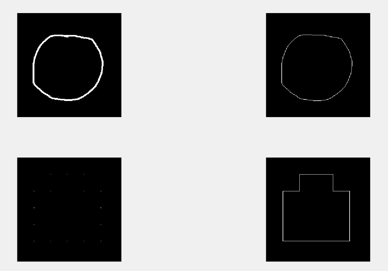
g为二值图像边界，g2为二次取样的边界，g3为连接g2的效果。

2.2 使用最小周长多边形的多边形近似

一条数字边界可由一个多边形以任意精度近似。对于一条闭合曲线,当多边形线段数目与边界点数目相同时，近似是精确的。因此，每一对相邻点定义了多边形的一条边。实践操作中，多边形近似的目的是用尽可能少的顶点表示边界的形状。
一种用于多边形近似的特殊方法是寻找一个区域或者一条边界的最小周长多边形(MPP)。
假设将图形看做“细胞联合体”即这个样子：（图中方块）

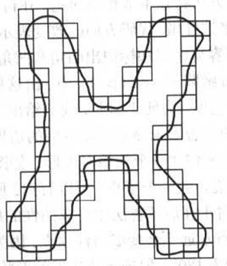
其最小周长多边形可以表示成（黑线部分）：

进一步可以表示为：

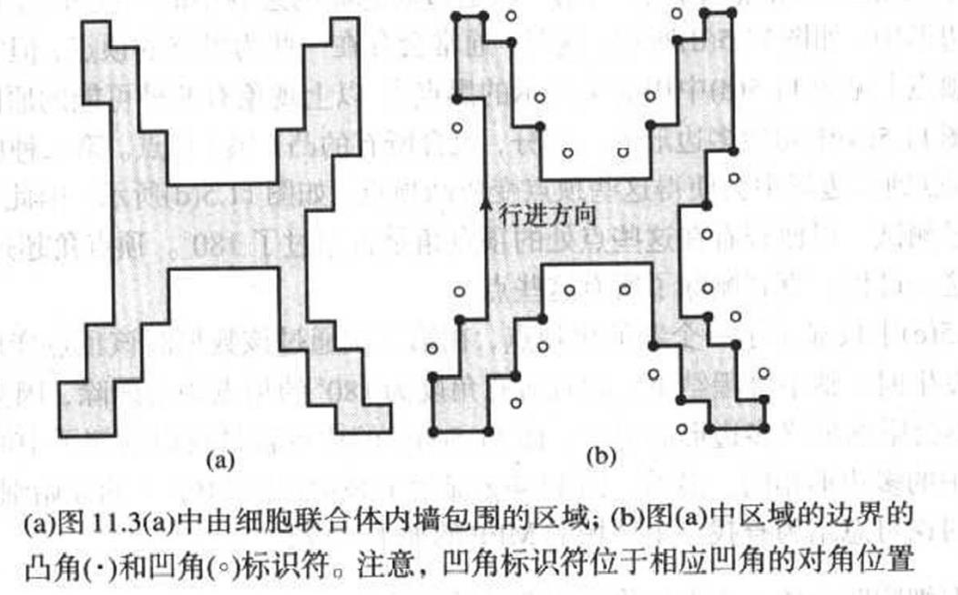
有以下基础结论：

1. 简单的细胞联合体MPP是本身不相交的。
2. MPP的每一个凸顶点用在上图中用黑点表示。（但不是所有黑点都是MPP的顶点）
3. MPP的每一个凹顶点用在上图中用白点表示。（但不是所有白点都是MPP的顶点）
4. 若一个黑点为MPP的一部分，且不是MPP的凸顶点，则其在MPP的边缘上。

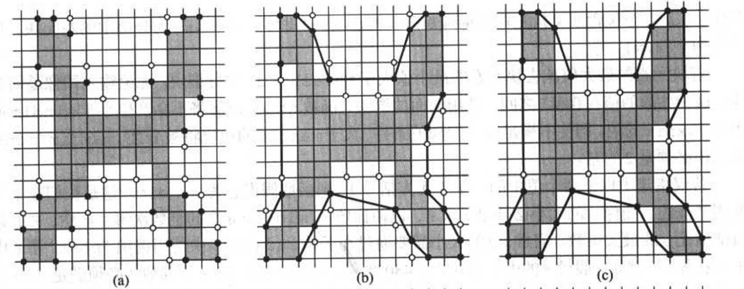
那么具体实现算法的过程可以按以下方式:

1. 获取细胞联合体
2. 获取细胞联合体的内部区域
3. 使用函数boundaries以四联接顺时针方式获取上一步中的区域边界
4. 使用函数fchcode获得该序列的Freeman链码
5. 从链码中获得凸顶点与凹顶点
6. 使用黑顶点构造一个初始多边形，再进一步的分析中删除位于该多边形之外的所有白顶点
7. 用剩余黑白顶点构造一个多边形
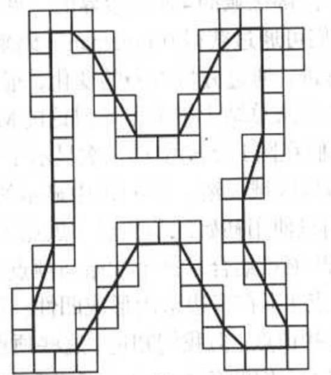
8. 删除所有为凹顶点的黑顶点
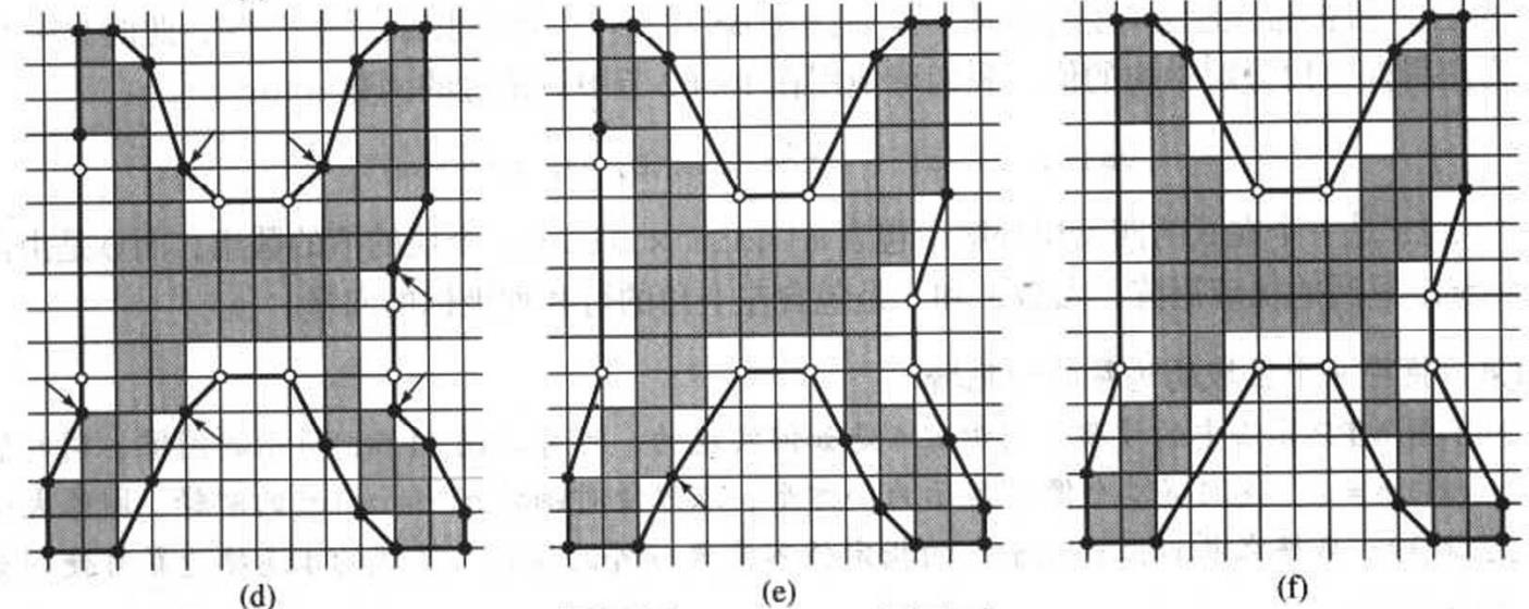
9. 重复7、8步，知道变化停止，且将所有角度为180°的顶点也删除，剩下的点就是MPP的顶点

可以用该图表示：

那么具体算法实现:

function [x, y] = minperpoly(B, cellsize)
%MINPERPOLY Computes the minimum perimeter polygon.
%   [X, Y] = MINPERPOLY(F, CELLSIZE) computes the vertices in [X, Y]
%   of the minimum perimeter polygon of a single binary region or
%   boundary in image B. The procedure is based on Slansky's
%   shrinking rubber band approach. Parameter CELLSIZE determines the
%   size of the square cells that enclose the boundary of the region
%   in B. CELLSIZE must be a nonzero integer greater than 1.
%   
%   The algorithm is applicable only to boundaries that are not
%   self-intersecting and that do not have one-pixel-thick
%   protrusions. 

%   Copyright 2002-2004 R. C. Gonzalez, R. E. Woods, & S. L. Eddins
%   Digital Image Processing Using MATLAB, Prentice-Hall, 2004
%   $Revision: 1.6 $  $Date: 2003/11/21 14:41:39 $

if cellsize <= 1
   error('CELLSIZE must be an integer > 1.'); 
end

% Fill B in case the input was provided as a boundary. Later 
% the boundary will be extracted with 4-connectivity, which 
% is required by the algorithm. The use of bwperim assures 
% that 4-connectivity is preserved at this point.               
B = imfill(B, 'holes');
B = bwperim(B);               
[M, N] = size(B);

% Increase image size so that the image is of size K-by-K
% with (a) K >= max(M,N) and (b)  K/cellsize = a power of 2.
K = nextpow2(max(M, N)/cellsize);
K = (2^K)*cellsize;
    
% Increase image size to nearest integer power of 2, by 
% appending zeros to the end of the image. This will allow 
% quadtree  decompositions as small as cells of size 2-by-2, 
% which is the smallest allowed value of cellsize.
M = K - M;
N = K - N;
B = padarray(B, [M N], 'post'); % f is now of size K-by-K

% Quadtree decomposition.
Q = qtdecomp(B, 0, cellsize); 

% Get all the subimages of size cellsize-by-cellsize.
[vals, r, c] = qtgetblk(B, Q, cellsize);

% Get all the subimages that contain at least one black 
% pixel. These are the cells of the wall enclosing the boundary.
I = find(sum(sum(vals(:, :, :)) >= 1));
x = r(I);
y = c(I);

% [x', y'] is a length(I)-by-2 array.  Each member of this array is
% the left, top corner of a black cell of size cellsize-by-cellsize.
% Fill the cells with black to form a closed border of black cells
% around interior points. These cells are the cellular complex.
for k = 1:length(I)
   B(x(k):x(k) + cellsize-1, y(k):y(k) + cellsize-1) = 1;
end
    
BF = imfill(B, 'holes');

% Extract the points interior to the black border. This is the region
% of interest around which the MPP will be found. 
B = BF & (~B);
    
% Extract the 4-connected boundary.
B = boundaries(B, 4, 'cw');
% Find the largest one in case of parasitic regions.
J = cellfun('length', B);
I = find(J == max(J));
B = B{I(1)};

% Function boundaries outputs the last coordinate pair equal to the
% first.  Delete it. 
B = B(1:end-1,:);
                  
% Obtain the xy coordinates of the boundary.
x = B(:, 1);
y = B(:, 2);

% Find the smallest x-coordinate and corresponding
% smallest y-coordinate.  
cx = find(x == min(x));
cy = find(y == min(y(cx)));

% The cell with top leftmost corner at (x1, y1) below is the first
% point considered by the algorithm.  The remaining points are
% visited in the clockwise direction starting at (x1, y1). 
x1 = x(cx(1));
y1 = y(cy(1));

% Scroll data so that the first point is (x1, y1).
I = find(x == x1 & y == y1);
x = circshift(x, [-(I - 1), 0]);
y = circshift(y, [-(I - 1), 0]);

% The same shift applies to B.
B = circshift(B, [-(I - 1), 0]);

% Get the Freeman chain code.  The first row of B is the required
% starting point. The first element of the code is the transition
% between the 1st and 2nd element of B, the second element of 
% the code is the transition between the 2nd and 3rd elements of B,
% and so on.  The last element of the code is the transition between
% the last and 1st elements of B. The elements of B form a cw
% sequence (see above), so we use 'same' for the direction in
% function fchcode. 
code = fchcode(B, 4, 'same'); 
code = code.fcc;

% Follow the code sequence to extract the Black Dots, BD, (convex
% corners) and White Dots, WD, (concave corners). The transitions are
% as follows: 0-to-1=WD; 0-to-3=BD; 1-to-0=BD; 1-to-2=WD; 2-to-1=BD;
% 2-to-3=WD; 3-to-0=WD; 3-to-2=dot.  The formula t = 2*first - second
% gives the following unique values for these transitions: -1, -3, 2,
% 0, 3, 1, 6, 4.  These are applicable to travel in the cw direction. 
% The WD's are displaced one-half a diagonal from the BD's to form
% the half-cell expansion required in the algorithm. 

% Vertices will be computed as array "vertices" of dimension nv-by-3,
% where nv is the number of vertices. The first two elements of any
% row of array vertices are the (x,y) coordinates of the vertex
% corresponding to that row, and the third element is 1 if the
% vertex is convex (BD) or 2 if it is concave (WD). The first vertex
% is known to be convex, so it is black. 
vertices = [x1, y1, 1];
n = 1;
k = 1;
for k = 2:length(code)
   if code(k - 1) ~= code(k)
      n = n + 1;
      t = 2*code(k-1) - code(k); % t = value of formula.
      if t == -3 | t == 2 | t == 3 | t == 4 % Convex: Black Dots.
         vertices(n, 1:3) = [x(k), y(k), 1];
      elseif t MATLAB数字图像处理学习笔记

 数字图像处理学习笔记之一 DIP绪论与MATLAB基础
 山东大学数字图像处理实验：MATLAB的图像显示方法
 Matlab中处理日期与时间的函数
 matlab学习记录
 数字图像处理(MATLAB版)学习笔记——第2章 灰度变换与空间滤波