总276 量化风险 004 金融时间序列分析

Posted 2021-05-02 量化金融科技前沿

第三章   金融时间序列分析的基础知识

chapter three - 1、2

1.Using the data in theworksheet named Question3.1 reproduce the moments and regression coefficientsat the bottom of Table 3.1.

2.Reproduce Figure3.1.

通过给定的自变量和因变量，分析它们的均值、方差以及相关系数和回归结果的截距以及自变量的系数。

代码如下：

def get_moments(df):
    ###  question one  moment 
    x_mean    =  df['x'].mean()
    x_var     =  df['x'].var()

    y_mean    =  df['y'].mean()
    y_var     =  df['y'].var()

    corre =df.corr()

    return x_mean,x_var,y_mean,y_var,corre    


def get_regression(df):
    ## regression
    arr_df = np.array(df)
    arr_df = arr_df.T
    x = np.array(arr_df[0])
    y = np.array(arr_df[1])

    x_total       = sm.add_constant(x)
    model         = sm.OLS(y,x_total)
    result        = model.fit()
    return result,result.summary(),result.params
dir = "/Users/chapter3/question1-1.xlsx"
df  = pd.read_excel(dir)
get_moments(df)
get_regression(df) 

可视化 -- 对比原始的散点图和回归结果：

代码如下：

##### 对比原始数据和回归结果的数据
def visual_result(df):
    ## regression
    arr_df = np.array(df)
    arr_df = arr_df.T
    x = np.array(arr_df[0])
    y = np.array(arr_df[1])
    x_total       = sm.add_constant(x)
    plt.scatter(x,y,alpha=0.3)
    model         = sm.OLS(y,x_total)
    result        = model.fit()

    #分别给x轴和y轴命名
    plt.xlabel("x")
    plt.ylabel("y")

    #添加回归线，红色
    y_hat=result.predict(x_total)
    plt.plot(x_total[:,1], y_hat, 'r', alpha=0.9) 

dir = "/Users/chapter3/question1-1.xlsx"
df  = pd.read_excel(dir)
visual_result(df)   

可视化结果如下：

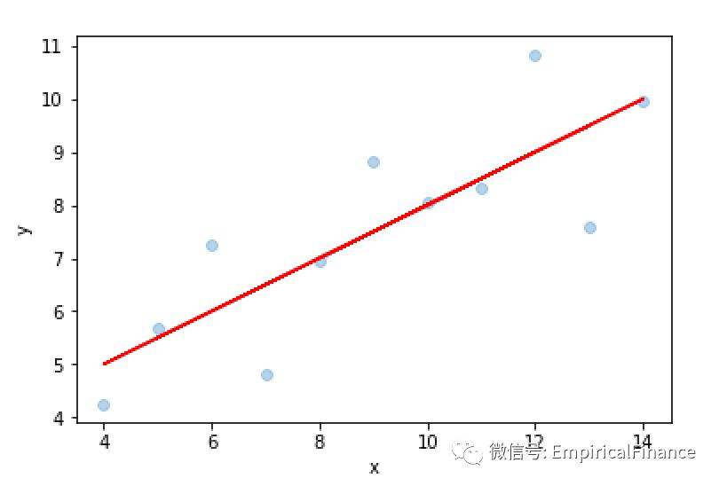
可以看出原始数据具有真正的线性关系；

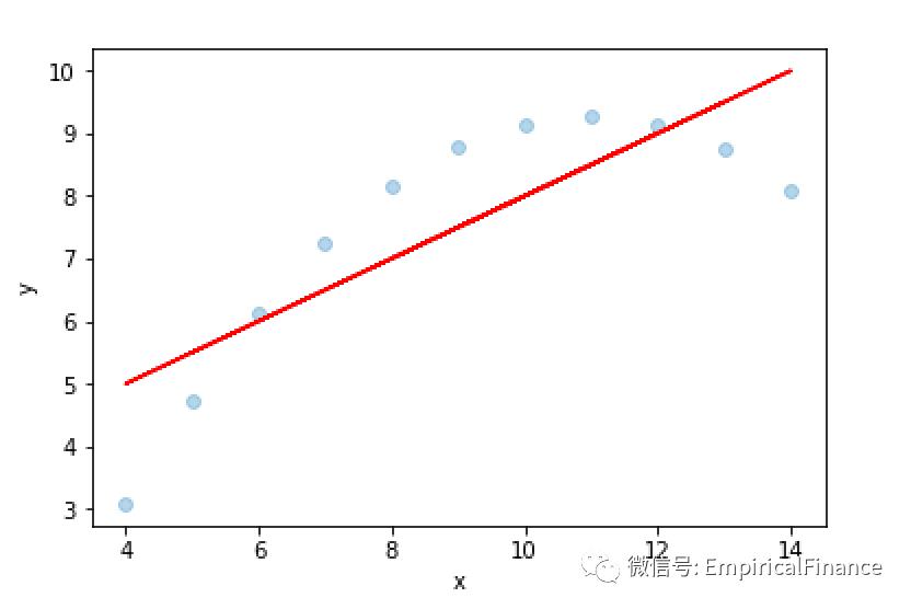原始数据具有非线性关系；

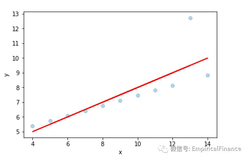
有偏估计，还具有异常值；

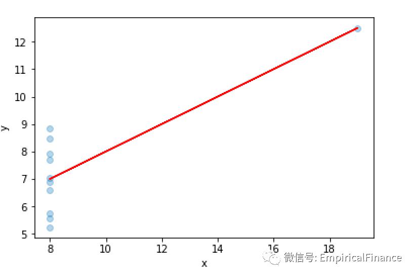
没有价值的关系，由于离群点而出现的线性关系

chapter three - 4

4.Using the data sets in the work sheet named Question3.4, estimate an AR(1)model on each of the 100 columns of data. (Excel hint: Use the LINEST function.) Plot the histogram of the 100 φ1 estimates you have obtained. The truevalue of φ1 is one in all the columns. What does the histogram tell you?

代码如下：

dir = "/Users/python/chapter3/question1-4.xlsx"
df  = pd.read_excel(dir)
paras_a = [] 
for i in range(100):
    x      = list(df[i+1].values)
    #### caculate the ACF
    mdl    = smt.AR(x).fit(maxlag=1, ic='aic', trend='nc')
    result = mdl.params[1]
    paras_a.append(result)

len(paras_a) 


# 参数依次为list,抬头,X轴标签,Y轴标签,XY轴的范围
def draw_hist(paras_a,Title,Xlabel,Ylabel,Xmin,Xmax,Ymin,Ymax):
   plt.hist(paras_a,100)
   plt.xlabel(Xlabel)
   plt.xlim(Xmin,Xmax)
   plt.ylabel(Ylabel)
   plt.ylim(Ymin,Ymax)
   plt.title(Title)
   plt.show()

draw_hist(paras_a,'Histogram of AR(1) Parameters','Area','number',0.76,1.05,0.05,9) 

结果如下：

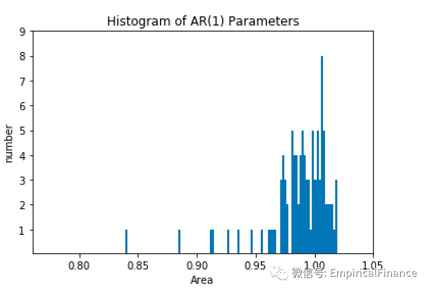
可以有一阶的自回归结果看出，测试的样本数据的一阶的回归系数取1左右的概率最大，也就是说数据当期和滞后一期的相关性很大。

以上是本期的全部内容，如有错误，望批评指出。

最后，祝大家周末愉快。

[指导老师：首都经济贸易大学  余颖丰；小编：北京第二外国语学院   李燕]