基于Tensorflow2.x低阶API搭建神经网络模型并训练及解决梯度爆炸与消失方法实践
Posted 肖永威
tags:
篇首语:本文由小常识网(cha138.com)小编为大家整理,主要介绍了基于Tensorflow2.x低阶API搭建神经网络模型并训练及解决梯度爆炸与消失方法实践相关的知识,希望对你有一定的参考价值。
1. 低阶API神经网络模型
1.1. 关于tf.Module
关于Tensorflow 2.x,最令我觉得有意思的功能就是tf.function和AutoGraph了.他们可以把Python风格的代码转为效率更好的Tensorflow计算图。
TensorFlow 2.0主要使用的是动态计算图和Autograph。Autograph机制可以将动态图转换成静态计算图,兼收执行效率和编码效率之利。
我们使用tf.Module来更好地构建Autograph。在介绍Autograph的编码规范时提到构建Autograph时应该避免在@tf.function修饰的函数内部定义tf.Variable。
但是如果在函数外部定义tf.Variable的话,又会显得这个函数有外部变量依赖,封装不够完美。
一种简单的思路是定义一个类,并将相关的tf.Variable创建放在类的初始化方法中。而将函数的逻辑放在其他方法中。
因此,TensorFlow提供了一个基类tf.Module,通过继承它构建子类,我们不仅可以获得以上的自然而然,而且可以非常方便地管理变量,还可以非常方便地管理它引用的其它Module,最重要的是,我们能够利用tf.saved_model保存模型并实现跨平台部署使用。
1.2. 全连接神经网络
全连接神经网络是人工神经网络中最简单的一种,中间每一个全连接层都会对输入节点乘上权重,然后加上一个bias,经过几层计算后通过一个激活函数输出节点,完成分类。
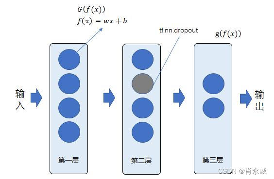
如图定义神经网络,其中 G ( f ( x ) ) G(f(x)) G(f(x))中 G G G函数采用relu函数, g ( f ( x ) ) g(f(x)) g(f(x))中 g g g函数采用多分类softmax函数。
1.3. 神经网络模型类的定义
layer=[2,32,32,2] #神经网络模型定义为4层全连接。
input_size = layer[0] #输入数据为2个

class DNNModel(tf.Module):
    def __init__(self, layer=[input_size,128,2], keep_prob = 0.2, name=None):
        super(DNNModel, self).__init__(name=name)
        self.layer=layer
        self.keep_prob = keep_prob
        self.num = len(self.layer)-1   # 网络层数
        self.w = []
        self.b = []
        h_in = self.layer[0]
        h_out = self.layer[1]

        for i in range(self.num):
            # tf.truncated_normal由tf.random.truncated_normal替换
            w0 = tf.Variable(tf.random.truncated_normal([h_in,h_out],stddev=0.1),name='weights' +str(i+1) )
            b0 = tf.Variable(tf.zeros([h_out],name='biases' + str(i+1)))
            self.w.append(w0)
            self.b.append(b0)
            if i < self.num -1:
                h_in = self.layer[i + 1]
                h_out = self.layer[i + 2]

        self.var = []
        for i in range(len(self.w)):
            self.var.append(self.w[i])
            self.var.append(self.b[i])

    #@tf.function(input_signature=[tf.TensorSpec(shape = [None,2], dtype = tf.float32)])
    @tf.function(input_signature=[tf.TensorSpec(shape = [None,input_size], dtype = tf.float32, name='dnn')])
    def __call__(self, x):
        x = tf.cast(x, tf.float32)  # 转换输入数据类型
        h1 = x
        for i in range(self.num):
            #定义前向传播过程
            if i < self.num -1:
                #h0 = tf.nn.relu(x@self.w[i] + self.b[i], name='layer' +str(i+1))
                h0 = tf.nn.relu(tf.matmul(h1, self.w[i]) + self.b[i], name='layer' +str(i+1))  # 或x@w,以及tf.add
                #使用dropout
                if i == 0:
                    h1 = h0
                else:
                    h1 = tf.nn.dropout(h0, rate = 1 - self.keep_prob)
            else:
                h1 = tf.matmul(h1, self.w[i]) + self.b[i]

        # 定义输出层
        self.y_conv = tf.nn.softmax(h1,name='y_conv')

        return self.y_conv

model = DNNModel(layer = layer, keep_prob = 0.2)  # 实例化模型类
tf.function本质上就是一个函数修饰器,它能够帮助将用户定义的python风格的函数代码转化成高效的tensorflow计算图(可以理解为:之前tf1.x中graph需要自己定义,现在tf.function能够帮助一起定义)。转换的这个过程称为AutoGraph。
我们使用input_signature对tf.function修饰的函数进行数字签名,其中,tf.TensorSpec() 函数签名由函数原型组成。它告诉你的是关于函数的一般信息,它的名称,参数,它的范围以及其他杂项信息。
tf.TensorSpec ( shape, dtype=tf.dtypes.float32, name=None )
注:对于被tf.function修饰过的函数都有get_concrete_function的属性,可以通过该操作对函数添加函数签名,从而获取特定追踪。通过增加函数签名之后才能够将模型保存。
将python标量或列表作为参数传递tf.function将始终建立一个新图形。为了避免这种情况,请尽可能将数字参数作为张量传递
2. 神经网络训练
2.1. 训练结构定义

2.2.1. 损失函数
交叉熵是分类问题中使用比较广的一种损失函数,刻画了两个概率分布之间的距离。给定两个概率分布 p p p和 q q q,通过 q q q来表示 p p p的交叉熵为:
H ( p , q ) = − ∑ x p ( x ) l o g q ( x ) H(p,q)=-\\sum_xp(x)logq(x) H(p,q)=−∑xp(x)logq(x)
交叉熵损失函数定义为:
l o s s = − ∑ i = 1 n y i l o g y ^ i loss=-\\sum_i=1^ny_ilog\\haty_i loss=−∑i=1nyilogy^i
其中, y ^ i \\haty_i y^i是预测值, y i y_i yi是实际值。
2.2.2. 训练类代码示例
class Train_Model(object):
    def __init__(self, model):
        self.model = model

    # 将预测值限制在 1e-10 以上, 1 - 1e-10 以下,避免log(0)错误
    def loss_func(self, y_true, y_pred, eps = 1e-10):
        y_pred = tf.clip_by_value(y_pred, eps, 1.0-eps)
        y_pred = tf.cast(y_pred, tf.float32)
        y_true = tf.cast(y_true, tf.float32)

        y_pred = - y_true*tf.math.log(y_pred) # 自定义交叉熵损失
        loss = tf.reduce_sum(tf.cast(y_pred, tf.float32))

        return loss

    # 计算准确度
    def metric_func(self, y_true, y_pred):
        preds = tf.argmax(y_pred, axis=1)  # 取值最大的索引,正好对应字符标签
        labels = tf.argmax(y_true, axis=1)
        accuracy = tf.reduce_mean(tf.cast(tf.equal(preds, labels), tf.float32))

        return accuracy
    # 训练输入,训练集X,训练集Y,测试集X,测试集Y,过程数,学习率,批次尺寸,最小值
    def train(self, X_train, Y_train, X_test, Y_test, EPOCHS, LEARNING_RATE=0.01, batch_size=32, eps = 1e-10):
        for epoch in tf.range(1,EPOCHS+1):
            i = 0
            for features, labels in data_iter(X_train, Y_train, batch_size):
                with tf.GradientTape() as tape:  # 追踪梯度
                    preds = self.model(features)
                    loss = self.loss_func(labels, preds, eps=eps)
                trainable_variables = self.model.var # 需优化参数列表
                grads = tape.gradient(loss, trainable_variables)  # 计算梯度,求导
                #梯度优化裁剪
                grads = [tf.clip_by_value(g, -0.5, 0.5) for g in grads if g is not None]
                optimizer = tf.optimizers.Adam(learning_rate=LEARNING_RATE)  # Adam 优化器
                optimizer.apply_gradients(zip(grads, trainable_variables))  # 更新梯度
                # 计算准确度
                accuracy = self.metric_func(labels, preds)
                # 输出各项指标
                if (i + 1) % 10 == 0:
                    print(f'Train: i, Train loss: loss, Test accuracy: accuracy')
                i = i + 1
            # 计算准确度
            y_pred = model(X_test)
            accuracy = self.metric_func(Y_test, y_pred)
            print('-----------------------------------')
            tf.print(f'Epoch [epoch/EPOCHS], Train loss: loss, Test accuracy: accuracy')

        return self.model

# 定义实例化训练类,输入神经网络模型
train = Train_Model(model)
2.2. 训练集及多分类one-hot编码
2.2.1. 训练集
按比例拆分(7/3)数据为训练集和测试,采用打乱Tensor索引方式,按索引抽取数据构建数据集。
使用tf.gather()按索引筛选数据集。
2.2.2. tf.one_hot()进行独热编码
独热编码(one-hot encoding)一般是在有监督学习中对数据集进行标注时候使用的,指的是在分类问题中,将分类数据转化为one-hot类型数据输出,相当于将多个数值联合放在一起作为多个相同类型的向量,可用于表示各自的概率分布,通常用于分类任务中作为最后的FC层的输出。
2.2.3. 代码及图示
这部分代码是本次实践过程的第一部分代码,在此引入所依赖的包。
import numpy as np
import pandas as pd
from matplotlib import pyplot as plt
import tensorflow as tf
%matplotlib inline
%config InlineBackend.figure_format = 'svg'
#正负样本数量
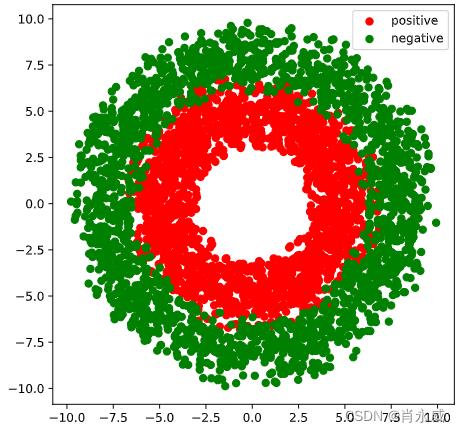
n_positive,n_negative = 2000,2000
#生成正样本, 小圆环分布
r_p = 5.0 + tf.random.truncated_normal([n_positive,1],0.0,1.0)
theta_p = tf.random.uniform([n_positive,1],0.0,2*np.pi)
Xp = tf.concat([r_p*tf.cos(theta_p),r_p*tf.sin(theta_p)],axis = 1)
Yp = tf.ones_like(r_p)
#生成负样本, 大圆环分布
r_n = 8.0 + tf.random.truncated_normal([n_negative,1],0.0,1.0)
theta_n = tf.random.uniform([n_negative,1],0.0,2*np.pi)
Xn = tf.concat([r_n*tf.cos(theta_n),r_n*tf.sin(theta_n)],axis = 1)
Yn = tf.zeros_like(r_n)
#汇总样本
X = tf.concat([Xp,Xn],axis = 0)
Y = tf.concat([Yp,Yn],axis = 0)
#多分类编码
lables = Y.numpy().reshape(-1)
Y = tf.one_hot(indices=lables, depth=2, on_value=1.0, off_value=0.0, axis=-1)
# 切分数据集,测试集占 30%
num_examples = len(X)
indices = list(range(num_examples))
np.random.shuffle(indices) #样本的读取顺序是随机的
split_size = int(num_examples*0.7)
indexs = indices[0: split_size]
X_train, Y_train = tf.gather(X,indexs), tf.gather(Y,indexs)
indexs = indices[split_size: num_examples]
X_test, Y_test = tf.gather(X,indexs), tf.gather(Y,indexs)
#可视化
plt.figure(figsize = (6,6))
plt.scatter(Xp[:,0].numpy(),Xp[:,1].numpy(),c = "r")
plt.scatter(Xn[:,0].numpy(),Xn[:,1].numpy(),c = "g")
plt.legend(["positive","negative"]);
2.3. 训练过程
- 训练样本训练过程为3次,EPOCHS=3;
- 学习率设置为,LEARNING_RATE=0.01;
- 训练输入每批次数据为,batch_size=16。
EPOCHS=3
LEARNING_RATE=0.01
batch_size=16
eps = 1e-10

train_model = train.train( X_train, Y_train, X_test, Y_test, EPOCHS, LEARNING_RATE=0.01, batch_size=32, eps = 1e-10)
训练过程如下:
	Train: 9, Train loss: 20.195472717285156, Test accuracy: 0.5625
	Train: 19, Train loss: 20.5467472076416, Test accuracy: 0.59375
	Train: 29, Train loss: 20.818161010742188, Test accuracy: 0.53125
	Train: 39, Train loss: 19.24681282043457, Test accuracy: 0.53125
	Train: 49, Train loss: 22.78866958618164, Test accuracy: 0.4375
	Train: 59, Train loss: 16.575977325439453, Test accuracy: 0.8125
	Train: 69, Train loss: 19.563919067382812, Test accuracy: 0.625
	Train: 79, Train loss: 18.80452537536621, Test accuracy: 0.6875
	Epoch [1/3], Train loss: 6.982160568237305, Test accuracy: 0.8075000047683716
	......
	Epoch [2/3], Train loss: 3.473015546798706, Test accuracy: 0.8600000143051147
	......
	Epoch [3/3], Train loss: 1.8749024868011475, Test accuracy: 0.9158333539962769
3. 梯度消失与梯度爆炸问题
梯度消失和梯度爆炸的根源主要是因为深度神经网络结构以及反向传播算法,在反向传播的过程中,需要对激活函数进行求导,如果导数大于1,那么会随着网络层数的增加梯度更新将会朝着指数爆炸的方式增加,这就是梯度爆炸。同样,如果导数小于1,那么随着网络层数的增加梯度更新信息会朝着指数衰减的方式减少,这就是梯度消失。
目前优化神经网络的方法都是基于反向传播的思想,即根据损失函数计算的误差通过反向传播的方式,指导深度网络权值的更新。
3.1. 简明通俗原理
通俗来讲,神经网络最基本节点的神经单元,数学表示为 y i = f ( w i x i + b i ) y_i=f(w_ix_i+b_i) yi=f(wixi+b基于Tensorflow2.x低阶API搭建神经网络模型并训练及解决梯度爆炸与消失方法实践
Python Tensorflow1.x升级到2.x低阶API实践
Python Tensorflow1.x升级到2.x低阶API实践
Python Tensorflow1.x升级到2.x低阶API实践