OpenCV从入门到入坟

Posted 2022-09-02 贪钱算法还我头发

tags:

篇首语：本文由小常识网(cha138.com)小编为大家整理，主要介绍了OpenCV从入门到入坟相关的知识，希望对你有一定的参考价值。

小脑一抽去学了狗都不学的CV，几天热度到现在全是凉水

学习视频链接b站openCV

1. 图像基本操作

1.1 图片处理

cv2.IMREAD_COLOR: 彩色图像
cv2.IMREAD_GRAYSCALE:灰度图像

import cv2  #opencv读取的格式的RGB
import matplotlib.pyplot as plt  # matplotlib的格式是RGB
import numpy as np
%matplotlib inline

图片读取

img = cv2.imread('img/cat.jpg')
print(img.shape)  # (414, 500, 3)
img
""
array([[[142, 151, 160],
        [146, 155, 164],
        [151, 160, 170],
        ...,
        [183, 198, 200],
        [128, 143, 145],
        [127, 142, 144]]], dtype=uint8)
""

def cv_show(name, img):
    cv2.imshow(name, img)
    cv2.waitKey(0)  # 等待时间，毫秒级，0表示任意键终止
    cv2.destroyAllWindows()

# 灰度图
img = cv2.imread('img/cat.jpg', cv2.IMREAD_GRAYSCALE)
print(img.shape, type(img), img.size, img.dtype)  # (414, 500) <class 'numpy.ndarray'> 207000 uint8
cv_show('image', img)
cv2.imwrite('img/mycat.jpg', img)

# 截取部分图像
cat = img[0:50, 0:200] 
cv_show('cat', cat)

# 颜色通道提取
img = cv2.imread('img/cat.jpg')
b, g, r = cv2.split(img)
print(r.shape) # (414, 500)
img = cv2.merge((b, g, r))
print(img.shape)  # (414, 500, 3)

# 只保留R
cur_img = img.copy()
cur_img[:,:,0] = 0
cur_img[:,:,1] = 0
cv_show('G', cur_img)

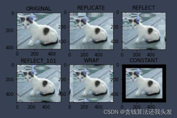
边界填充

BORDER_REPLICATE：复制最边缘像素
BORDER_REFLECT：反射法，对感兴趣的图像中的像素在两边进行复制例如：fedcba|abcdefgh|hgfedcb
BORDER_REFLECT_101：反射法，也就是以最边缘像素为轴，对称，gfedcb|abcdefgh|gfedcba
BORDER_WRAP：外包装法cdefgh|abcdefgh|abcdefg
BORDER_CONSTANT：常量法，常数值填充

top_size, bottom_size, left_size, right_size = (50, 50, 50, 50)
replicate = cv2.copyMakeBorder(img, top_size, bottom_size, left_size, right_size, borderType=cv2.BORDER_REPLICATE)
reflect = cv2.copyMakeBorder(img, top_size, bottom_size, left_size, right_size, borderType=cv2.BORDER_REFLECT)
reflect101 = cv2.copyMakeBorder(img, top_size, bottom_size, left_size, right_size, borderType=cv2.BORDER_REFLECT_101)
wrap = cv2.copyMakeBorder(img, top_size, bottom_size, left_size, right_size, borderType=cv2.BORDER_WRAP)
constant = cv2.copyMakeBorder(img, top_size, bottom_size, left_size, right_size, borderType=cv2.BORDER_CONSTANT, value=0)
plt.subplot(231), plt.imshow(img, 'gray'), plt.title('ORIGINAL')
plt.subplot(232), plt.imshow(replicate, 'gray'), plt.title('REPLICATE')
plt.subplot(233), plt.imshow(reflect, 'gray'), plt.title('REFLECT')
plt.subplot(234), plt.imshow(reflect101, 'gray'), plt.title('REFLECT_101')
plt.subplot(235), plt.imshow(wrap, 'gray'), plt.title('WRAP')
plt.subplot(236), plt.imshow(constant, 'gray'), plt.title('CONSTANT')
plt.show()

数值计算

img_cat = cv2.imread('img/cat.jpg')
img_cat2 = img_cat + 10 
print(img_cat[:5,:,0])
print(img_cat2[:5,:,0])
""
[[142 146 151 ... 156 155 154]
 [108 112 118 ... 155 154 153]
 [108 110 118 ... 156 155 154]
 [139 141 148 ... 156 155 154]
 [153 156 163 ... 160 159 158]]
[[152 156 161 ... 166 165 164]
 [118 122 128 ... 165 164 163]
 [118 120 128 ... 166 165 164]
 [149 151 158 ... 166 165 164]
 [163 166 173 ... 170 169 168]]
""

print((img_cat + img_cat2)[:5,:,0]) # 相当于% 256
print(cv2.add(img_cat, img_cat2)[:5, :, 0]) # 超过的赋值为最大值
""
[[ 38  46  56 ...  66  64  62]
 [226 234 246 ...  64  62  60]
 [226 230 246 ...  66  64  62]
 [ 32  36  50 ...  66  64  62]
 [ 60  66  80 ...  74  72  70]]
[[255 255 255 ... 255 255 255]
 [226 234 246 ... 255 255 255]
 [226 230 246 ... 255 255 255]
 [255 255 255 ... 255 255 255]
 [255 255 255 ... 255 255 255]]
""

图像融合

img_cat = cv2.imread('img/cat.jpg')
img_dog = cv2.imread('img/dog.jpg')
img_cat + img_dog
""
---------------------------------------------------------------------------
ValueError                                Traceback (most recent call last)
<ipython-input-30-e16b258924d3> in <module>
      1 img_cat = cv2.imread('img/cat.jpg')
      2 img_dog = cv2.imread('img/dog.jpg')
----> 3 img_cat + img_dog

ValueError: operands could not be broadcast together with shapes (414,500,3) (429,499,3) 
""

img_dog = cv2.resize(img_dog, (500, 414))
print(img_dog.shape)  # (414, 500, 3)
res = cv2.addWeighted(img_cat, 0.4, img_dog, 0.6, 0)
plt.imshow(res)

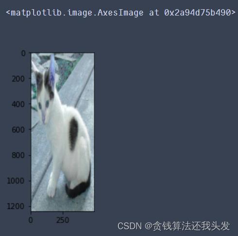
res = cv2.resize(img_cat, (0, 0), fx=4, fy=4)
plt.imshow(res)

res = cv2.resize(img, (0, 0), fx=1, fy=3)
plt.imshow(res)

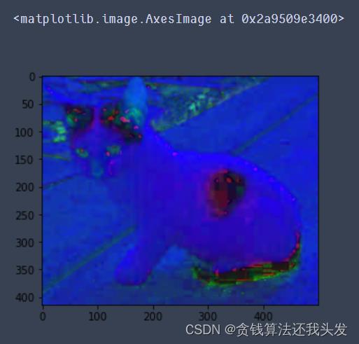
HSV

H - 色调（主波长）
S - 饱和度（纯度/颜色的阴影）
V值（强度）

# gray = cv2.cvtColor(img,cv2.COLOR_BGR2GRAY) # 灰度图
hsv = cv2.cvtColor(img_cat, cv2.COLOR_BGR2HSV)
plt.imshow(hsv)

图像阈值

ret, dst = cv2.threshold(src, thresh, maxval, type)

src：输入图，只能输入单通道图像，通常来说为灰度图
dst：输出图
thresh：阈值
maxval：当像素值超过了阈值（或者小于阈值，根据type来决定），所赋予的值
type：二值化操作的类型，包含以下5种类型：
- cv2.THRESH_BINARY: 超过阈值部分取maxval（最大值），否则取0
- cv2.THRESH_BINARY_INV: THRESH_BINARY的反转
- cv2.THRESH_TRUNC: 大于阈值部分设为阈值，否则不变
- cv2.THRESH_TOZERO: 大于阈值部分不改变，否则设为0
- cv2.THRESH_TOZERO_INV: THRESH_TOZERO的反转

img_gray = cv2.cvtColor(img_cat, cv2.COLOR_BGR2GRAY)
ret, thresh1 = cv2.threshold(img_gray, 127, 255, cv2.THRESH_BINARY)
ret, thresh2 = cv2.threshold(img_gray, 127, 255, cv2.THRESH_BINARY_INV)
ret, thresh3 = cv2.threshold(img_gray, 127, 255, cv2.THRESH_TRUNC)
ret, thresh4 = cv2.threshold(img_gray, 127, 255, cv2.THRESH_TOZERO)
ret, thresh5 = cv2.threshold(img_gray, 127, 255, cv2.THRESH_TOZERO_INV)

titles = ['Original Image', 'BINARY', 'BINARY_INV', 'TRUNC', 'TOZERO', 'TOZERO_INV']
images = [img, thresh1, thresh2, thresh3, thresh4, thresh5]

for i in range(6):
    plt.subplot(2, 3, i + 1), plt.imshow(images[i], 'gray')
    plt.title(titles[i])
#     plt.xticks([]), plt.yticks([])
plt.show()

图像平滑

img = cv2.imread('img/lenaNoise.png')
cv_show('img', img)

# 均值滤波：简单的卷积操作
blur =  cv2.blur(img, (3, 3))
cv_show('blur', blur)

# 方框滤波： 基本和均值一样，可以选择归一化
box = cv2.boxFilter(img, -1, (3, 3), normalize=True)
cv_show('box', box)

# 高斯滤波：高斯模糊的卷积核里的数值是满足高斯分布，相当于更重视中间的
aussian = cv2.GaussianBlur(img, (5, 5), 1)
cv_show('aussian', aussian)

# 中值滤波：相当于用中值代替
median = cv2.medianBlur(img, 5)
cv_show('median', median)

# 展示所有的
res = np.hstack((blur, aussian, median))
cv_show('res', res)

形态学-腐蚀操作

img = cv2.imread('img/dige.png')
cv_show('img', img)
kernal = np.ones((3, 3), np.uint8)
erosion = cv2.erode(img, kernal, iterations=1)
cv_show('erosion', erosion)

pie = cv2.imread('img/pie.png')
cv_show('pie', pie)
kernel = np.ones((30, 30),np.uint8) 
erosion_1 = cv2.erode(pie, kernel, iterations = 1)
erosion_2 = cv2.erode(pie, kernel, iterations = 2)
erosion_3 = cv2.erode(pie, kernel, iterations = 3)
res = np.hstack((erosion_1 erosion_2, erosion_3))
cv_show('res', res)

形态学-膨胀操作

img = cv2.imread('img/dige.png')
cv_show('img', img)
kernel = np.ones((3, 3), np.uint8) 
dige_erosion = cv2.erode(img, kernel, iterations = 1)
dige_dilate = cv2.dilate(dige_erosion, kernel, iterations = 1) # 腐蚀膨胀后不变
cv_show('dige_dilate', dige_dilate)

pie = cv2.imread('img/pie.png')
cv_show('pie', pie)
kernel = np.ones((30,30),np.uint8) 
dilate_1  = cv2.dilate(pie, kernel, iterations = 1)
dilate_2  = cv2.dilate(pie, kernel, iterations = 2)
dilate_3  = cv2.dilate(pie, kernel, iterations = 3)
res = np.hstack((dilate_1, dilate_2, dilate_3))
cv_show('res', res)

开运算与闭运算

img = cv2.imread('img/dige.png')
kernel = np.ones((5, 5), np.uint8) 
# 开：先腐蚀，再膨胀
opening = cv2.morphologyEx(img, cv2.MORPH_OPEN, kernel)
# 闭：先膨胀，再腐蚀
closing = cv2.morphologyEx(img, cv2.MORPH_CLOSE, kernel)
res = np.hstack((img, opening, closing))
cv_show('res', res)

梯度运算

# 梯度 = 膨胀 - 腐蚀
pie = cv2.imread('img/pie.png')
kernel = np.ones((7, 7), np.uint8) 
dilate = cv2.dilate(pie, kernel, iterations = 5)
erosion = cv2.erode(pie, kernel, iterations = 5)
gradient = cv2.morphologyEx(pie, cv2.MORPH_GRADIENT, kernel)
res = np.hstack((pie, dilate, erosion, gradient))
cv_show('res', res)

礼帽与黑帽

礼帽 = 原始输入- 开运算结果
黑帽 = 闭运算 - 原始输入

img = cv2.imread('img/dige.png')
tophat = cv2.morphologyEx(img, cv2.MORPH_TOPHAT, kernel)
blackhat  = cv2.morphologyEx(img, cv2.MORPH_BLACKHAT, kernel)
res = np.hstack((img, tophat, blackhat))
cv_show('res', res)

图像梯度-Sobel算子

dst = cv2.Sobel(src, ddepth, dx, dy, ksize)

ddepth:图像的深度
dx和dy分别表示水平和竖直方向
ksize是Sobel算子的大小

img = cv2.imread('img/pie.png',cv2.IMREAD_GRAYSCALE)
sobelx = cv2.Sobel(img, cv2.CV_64F, 1, 0, ksize=3)
res = np.hstack((img, sobelx))
cv_show(Spring Boot 2从入门到入坟 | 基础入门篇：「Spring Boot 2从入门到入坟」系列教程介绍
 超全面的线段树：从入门到入坟
 数据库从入门到入坟
 《HTML从入门到入坟》第一期
 Spring Boot 2从入门到入坟 | 自动配置篇：源码分析之自动配置流程
 Java从入门到入坟系列学习路线目录索引（持续更新中~~~）