Keras深度学习实战(15)——从零开始实现YOLO目标检测
Posted 盼小辉丶
tags:
篇首语:本文由小常识网(cha138.com)小编为大家整理,主要介绍了Keras深度学习实战(15)——从零开始实现YOLO目标检测相关的知识,希望对你有一定的参考价值。
Keras深度学习实战(15)——从零开始实现YOLO目标检测
0. 前言
在《从零开始实现R-CNN目标检测》中我们学习了 R-CNN 目标检测模型,但基于候选区域的卷积神经网络目标检测 (例如 R-CNN 等) 的缺点之一是,由于选择性搜索需要花费大量时间获取候选区域,因此它无法实现实时目标检测。这导致基于候选区域的目标检测算法在诸如自动驾驶这类需要实时检测的应用中无法使用。
为了实现实时检测,我们将实现另一类主流目标检测模型 YOLO (You Only Look Once),该模型仅需要对图像进行一次运算,即可识别图像中目标对象,并在图像中对象周围绘制边框。
1. YOLO目标检测模型
要了解 YOLO 如何克服在生成候选区域时耗费大量时间的弊端,我们首先需要对 YOLO 目标检测模型进行分解介绍。
接下来,我们将通过使用 YOLO 的单次向前传递进行目标检测预测任务,包括预测图像中的对象类别及其边界框,并将其与我们在《从零开始实现R-CNN目标检测》中上一节实现的基于候选区域的 R-CNN 算法进行比较。
1.1 锚框 (anchor boxes)
为了了解 YOLO 的工作细节,让我们首先使用一个简单示例进行讲解。假设输入图像如下所示,其中图像被分为 3 x 3 的网格:
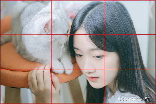
在这种情况下,神经网络模型的输出大小应为 3 x 3 x 5,其中 3 x 3 对应于图像中网格的数量,输出中的 5 的第一个输出表示对应网格是否包含目标对象,其他四个组成部分是与图像中网格相对应实际对象边界框的 x、y、w 和 h的偏移。
YOLO 目标检测模型中另一个重要概念是锚框 (anchor boxes)。我们知道图像中的边界框都具有不同形状比例,例如,汽车的边界框宽度大于高度,而人的边界框宽度通常小于高度。因此,我们可以将图像集中所有不同比例的边界框聚类为五个簇,这会产生五个具有不同高度和宽度的矩形框,我们将它们称为锚框,可以使用这些锚框来标识图像中对象周围的边界框。
如果在图像上有五个锚框,则输出相应的变为 3 x 3 x 5 x 5,其中 5 x 5 对应于五个锚框中对象类别概率和图像中锚框相对应实际对象边界框的 x、y、w 和 h 的偏移量,而 3 x 3 x 5 x 5 的输出可以通过神经网络模型的一次前向传播完成。
接下来,我们介绍如何得到锚框尺寸:
- 提取数据集中所有图像的宽度和高度
- 使用具有
5个聚类核的k 均值聚类,以聚类图像中存在的对象边界框宽度和高度 - 五个聚类中心对应于用于构建模型的五个锚框的宽度和高度
1.2 YOLO 目标检测模型原理
了解的锚框的基本概念以及如何获取锚框后,我们继续介绍 YOLO 算法的原理:
- 将图像划分为固定数量的网格单元
- 与图像中目标的真实边界框中心相对应的网格负责预测目标边界框
- 锚框的中心应与网格的中心相同
- 创建训练数据集:
- 对于包含对象中心的网格,其类别标签为
1,并且需要为每个锚点框计算x、y、w和h的偏移量 - 对于不包含对象中心的网格,其类别标签为
0,其x、y、w和h的偏移量则无关紧要
- 对于包含对象中心的网格,其类别标签为
- 在第一个模型中,我们将预测包含图像中心的锚框和网格单元组合
- 在第二个模型中,我们预测锚框的边界框偏移量
下一节中,我们将从零开始构建用于执行人物目标检测的深度神经网络模型。
2. 从零开始实现 YOLO 目标检测
我们继续使用在《R-CNN 目标检测模型》中使用的数据集,其中包含图像中目标对象类别以及相应边界框坐标,其详细介绍参考《从零开始实现R-CNN目标检测》。
2.1 加载数据集
导入相关的库,并定义相关数据集目录:
import json, scipy, os, time
import sys, cv2, xmltodict
import matplotlib.pyplot as plt
import numpy as np
import pandas as pd
import gc, scipy, argparse
from copy import deepcopy
# 数据集目录
xmls_root ="VOCtrainval_11-May-2012/VOCdevkit/VOC2012/"
annotations = xmls_root + "Annotations/"
jpegs = xmls_root + "JPEGImages/"
XMLs = os.listdir(annotations)
# 网格超参数
num_grids = 5
print(XMLs[:10])
print(len(XMLs))

file_name = '8.png'
# 数据集查看
ix = np.random.randint(len(XMLs))
sample_xml = XMLs[ix]
sample_xml = '/'.format(annotations, sample_xml)
with open(sample_xml, "rb") as f:    # notice the "rb" mode
    d = xmltodict.parse(f, xml_attribs=True)
print(d)
定义交并比 (Intersection over Union, IoU) 计算函数:
def calc_iou(candidate, current_y, img_shape):
    boxA = deepcopy(candidate)
    boxB = deepcopy(current_y)
    boxA[2] += boxA[0]
    boxA[3] += boxA[1]
    iou_img1 = np.zeros(img_shape)
    iou_img1[int(boxA[1]):int(boxA[3]), int(boxA[0]):int(boxA[2])] = 1
    iou_img2 = np.zeros(img_shape)
    iou_img2[int(boxB[1]):int(boxB[3]), int(boxB[0]):int(boxB[2])] = 1
    iou = np.sum(iou_img1*iou_img2) / (np.sum(iou_img1) + np.sum(iou_img2) - np.sum(iou_img1*iou_img2))
    return iou
2.2 计算锚框尺寸
将锚框的宽度和高度归一化为图像宽度和高度的百分比,以保证在图像缩放时,锚框的百分比并不会改变。
在边界框中标识人物所有可能的宽度和高度锚框,遍历所有的图像,记录只包括一个人物对象的图片,并解析计算边界框的宽度和高度:
y_train = []

for i in XMLs[:10000]:
    xml_file = annotations + i
    arg1 = i.split('.')[0]
    with open(xml_file, 'rb') as f:
        d = xmltodict.parse(f, xml_attribs=True)
        l = []
        if type(d['annotation']['object']) == type(l):
            discard = 1
        else:
            x1 = ((float(d['annotation']['object']['bndbox']['xmin'])))/(float(d['annotation']['size']['width']))
            x2 = ((float(d['annotation']['object']['bndbox']['xmax'])))/(float(d['annotation']['size']['width']))
            y1 = ((float(d['annotation']['object']['bndbox']['ymin'])))/(float(d['annotation']['size']['height']))
            y2 = ((float(d['annotation']['object']['bndbox']['ymax'])))/(float(d['annotation']['size']['height']))
            cls = d['annotation']['object']['name']
            if cls == 'person':
                y_train.append([x2-x1, y2-y1])
使用具有五个聚类中心的 k 均值聚类拟合边界框的宽度和高度,得到五个聚类中心作为锚框:
y_train = np.array(y_train)
from sklearn.cluster import KMeans

km = KMeans(n_clusters=5)
km.fit(y_train)
anchors = np.array(km.cluster_centers_).tolist()
print(km.cluster_centers_)
得到的聚类中心的结果如下所示:
[[0.84231561 0.89869485]
 [0.16385373 0.29783605]
 [0.2713572  0.61432026]
 [0.55194672 0.57477447]
 [0.48429325 0.86908945]]
2.3 创建训练数据集
(1) 初始化空列表,以便可以在进一步处理中记录数据:
k = -1
pre_xtrain = []
y_train = []
cls = []
xtrain = []
final_cls = []
dx = []
dy = []
dw = []
dh = []
final_delta = []
av = 0
x_train = []
y_delta = []
anc = []
(2) 遍历数据集,为了简单起见,我们仅使用包含一个对象并且该对象是人物的图像:
for i in XMLs[:10000]:
    xml_file = annotations + i
    arg1 = i.split('.')[0]
    discard=0
    with open(xml_file, "rb") as f:
        d = xmltodict.parse(f, xml_attribs=True)
        l = []
        ## 仅使用包含一个对象并且该对象是人物的图像
        if type(d["annotation"]["object"]) == type(l):
            discard = 1
        else:
            coords = arg1:[]
            pre_xtrain.append(arg1)
            m = pre_xtrain[(k+1)]
            k = k+1
        if(discard==0):
            x1=((float(d['annotation']['object']['bndbox']['xmin'])))/(float(d['annotation']['size']['width']))
            x2=((float(d['annotation']['object']['bndbox']['xmax'])))/(float(d['annotation']['size']['width']))
            y1=((float(d['annotation']['object']['bndbox']['ymin'])))/(float(d['annotation']['size']['height']))
            y2=((float(d['annotation']['object']['bndbox']['ymax'])))/(float(d['annotation']['size']['height']))
            cls=d['annotation']['object']['name']
            if(cls == 'person'):
                coords[arg1].append(x1)
                coords[arg1].append(y1)
                coords[arg1].append(x2)
                coords[arg1].append(y2)
                coords[arg1].append(cls)
在以上代码中,获取了归一化后的对象位置(使用图像的宽度和高度进行归一化)。
(3) 调整人物图像的大小,以使所有图像都具有相同的形状。此外,使用 preprocess_input 函数对图像进行预处理,以使其满足vgg16模型的输入需求:
                filename = jpegs + arg1 + '.jpg'
                img_size = 224
                img = cv2.imread(filename)
                img2 = cv2.resize(img,(img_size,img_size))
                img2 = preprocess_input(img2.reshape(1, 224, 224, 3))
(4) 提取对象边界框位置以及在缩放后的图像中的边界框坐标:
               # 对象在缩放后的图像中的位置
                current_y = [int(x1*224), int(y1*224), int(x2*224), int(y2*224)]
                label_center = [(current_y[0]+current_y[2])/2,(current_y[1]+current_y[3])/2]
                label = current_y
                # 对象在原图像中的位置坐标
                current_y2 = [float(d['annotation']['object']['bndbox']['xmin']),
                                float(d['annotation']['object']['bndbox']['ymin']),
                                float(d['annotation']['object']['bndbox']['xmax'])-float(d['annotation']['object']['bndbox']['xmin']),
                                float(d['annotation']['object']['bndbox']['ymax'])-float(d['annotation']['object']['bndbox']['ymin'])]
(5) 使用预训练的 VGG16 提取输入图像特征:
                vgg_predict = vgg16_model.predict(img2)
                x_train.append(vgg_predict)
(6) 通过以上步骤,我们已经完成了创建输入特征。接下来,创建训练集输出,由于我们将图片划分为 5 x 5 的网格,每个网格包含 5 个锚框,因此需要为类别预测提供 5 x 5 x 5 的输出,为边界框偏移预测提供 5 x 5 x 20 的输出。
首先,为目标类别标签和边界框偏移初始化数组:
                target_class = np.zeros((num_grids,num_grids,5))
                target_delta = np.zeros((num_grids,num_grids,20))
接下来,定义一个计算包含对象中心网格的函数:
def positive_grid_cell(label,img_width = 224, img_height = 224):
    label_center = [(label[0]+label[2])/(2),(label[1]+label[3])/(2)]
    a = int(label_center[0]/(img_width/num_grids))
    b = int(label_center[1]/(img_height/num_grids))
    return a, b
使用以上函数,我们为包含对象中心的网格分配标签类别 1,并且所有其它网格的标签都为 0。
a,b = positive_grid_cell(label)
接下来,我们定义另外一个函数,该函数用于查找最接近目标对象边界框的锚框:
def find_closest_anchor(label,img_width, img_height):
    label_width = (label[2]-label[0])/img_width
    label_height = (label[3]-label[1])/img_height
    label_width_height_array = np.array([label_width, label_height])
    distance = np.sum(np.square(np.array(anchors) - label_width_height_array), axis=1)
    closest_anchor = anchors[np.argmin(distance)]
    return closest_anchor
find_closest_anchor 函数将图像中目标对象的宽度和高度与所有可能的锚框进行比较,并标识最接近图像中实际对象宽度和高度的锚框。
最后,我们定义一个计算锚框与目标边界框偏移的函数 closest_anchor_corrections:
def closest_anchor_corrections(a, b, anchor, label, img_width, img_height):
    label_center = [(label[0]+label[2])/(2),(label[1]+label[3])/(2)]
    anchor_center = [a*img_width/num_grids , b*img_height/num_grids]
    dx = (label_center[0] - anchor_center[0])/img_width
    dy = (label_center[1] - anchor_center[1])/img_height
    dw = ((label[2] - label[0])/img_width) / (anchor[0])
    dh = ((label[3] - label[1])/img_height) / (anchor[1])
    return dx, dy, dw, dh
编写相关函数后,我们继续创建目标检测模型目标输出数据:
for a2 in range(num_grids):
for b2 in range(num_grids):
for m in range(len(anchors)):
dx, dy, dw, dh = closest_anchor_corrections(a2, b2, anchors[m], label, 224, 224)
target_class[a2,b2