《深度学习入门 基于Python的理论与实现》书中代码笔记

Posted 2022-04-02 海轰Pro

源码笔记【仅为个人笔记记录】

第三章

sigmoid函数

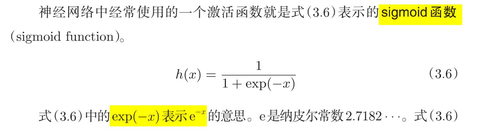
# coding: utf-8
import numpy as np
import matplotlib.pylab as plt


def sigmoid(x):
    return 1 / (1 + np.exp(-x))    

X = np.arange(-5.0, 5.0, 0.1)
Y = sigmoid(X)

plt.plot(X, Y)
plt.ylim(-0.1, 1.1)
plt.show()

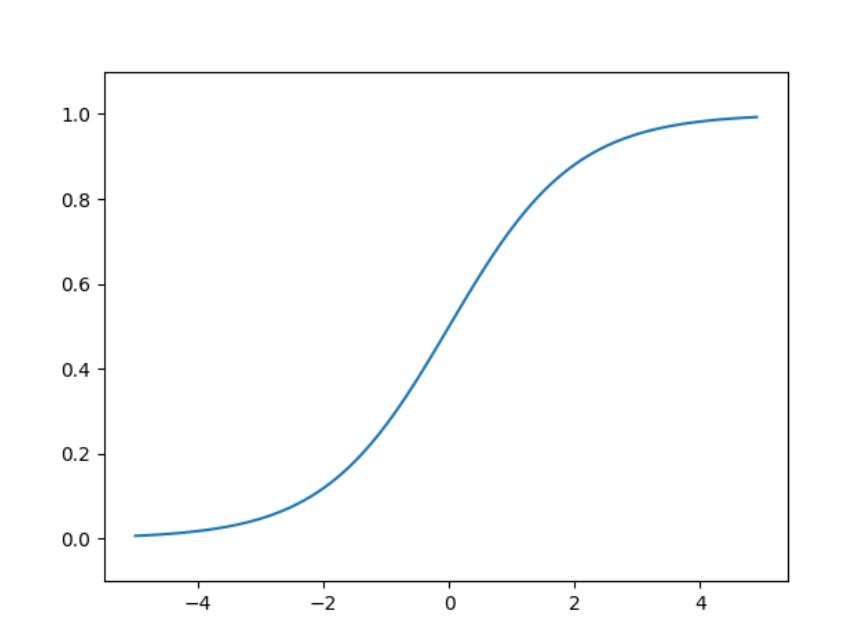
阶跃函数

# coding: utf-8
import numpy as np
import matplotlib.pylab as plt


def step_function(x):
    return np.array(x > 0, dtype=int)


X = np.arange(-5.0, 5.0, 0.1)
Y = step_function(X)
plt.plot(X, Y)
plt.ylim(-0.1, 1.1)  # 指定图中绘制的y轴的范围
plt.show()

ReLU函数

# coding: utf-8
import numpy as np
import matplotlib.pylab as plt


def relu(x):
    return np.maximum(0, x)


x = np.arange(-5.0, 5.0, 0.1)
y = relu(x)

plt.plot(x, y)
plt.ylim(-1.0, 5.5)
plt.show()

MNIST数据集的显示

# coding: utf-8

import numpy as np
from dataset.mnist import load_mnist
from PIL import Image

import sys
import os
sys.path.append(os.pardir)  # 为了导入父目录的文件而进行的设定


def img_show(image):
    pil_img = Image.fromarray(np.uint8(image))
    pil_img.show()


(x_train, t_train), (x_test, t_test) = load_mnist(flatten=True, normalize=False)

# 读取训练集中的第一张图片
img = x_train[0]
# 读取训练集中的第一张图片的标签
label = t_train[0]
print(label)  # 5

print(img.shape)  # (784,)
img = img.reshape(28, 28)  # 把图像的形状变为原来的尺寸
print(img.shape)  # (28, 28)

img_show(img)

使用已训练好的参数进行手写数字图片的预测

# coding: utf-8
import numpy as np
import pickle
from dataset.mnist import load_mnist
from common.functions import sigmoid, softmax

import sys
import os
sys.path.append(os.pardir)  # 为了导入父目录的文件而进行的设定


# 获取训练、测试数据
# x:图片
# t:标签
def get_data():
    (x_train, t_train), (x_test, t_test) = load_mnist(normalize=True, flatten=True, one_hot_label=False)
    return x_test, t_test

# 获取已训练好的网络参数
def init_network():
    with open("sample_weight.pkl", 'rb') as f:
        network = pickle.load(f)
    return network


# 进行图片的预测
def predict(network, x):
    # 参数设置
    W1, W2, W3 = network['W1'], network['W2'], network['W3']
    b1, b2, b3 = network['b1'], network['b2'], network['b3']

    # 输入 + 两层层隐藏层 + 输出层
    # 输入 1 * 784 (784 = 28 * 28)
    # 第一层 50个神经元 784 * 50
    # 第二层 100个神经元 50 * 100
    # 输出层 10个神经元 100 * 10
    a1 = np.dot(x, W1) + b1
    z1 = sigmoid(a1)
    a2 = np.dot(z1, W2) + b2
    z2 = sigmoid(a2)
    a3 = np.dot(z2, W3) + b3
    y = softmax(a3)

    # 返回一个1*10的数组
    # 表示10个分类对应的概率
    return y


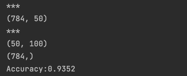
x, t = get_data()
network = init_network()
print("***")
print(network['W1'].shape)
print("***")
print(network['W2'].shape)
accuracy_cnt = 0
print(x[0].shape)
for i in range(len(x)):
    y = predict(network, x[i])
    p= np.argmax(y) # 获取概率最高的元素的索引
    if p == t[i]:
        accuracy_cnt += 1

print("Accuracy:" + str(float(accuracy_cnt) / len(x)))

使用已训练好的参数进行手写数字图片的预测（批处理）

区别：每次预测是使用多个图片同时进行预测

# coding: utf-8
import sys, os
sys.path.append(os.pardir)  # 为了导入父目录的文件而进行的设定
import numpy as np
import pickle
from dataset.mnist import load_mnist
from common.functions import sigmoid, softmax


def get_data():
    (x_train, t_train), (x_test, t_test) = load_mnist(normalize=True, flatten=True, one_hot_label=False)
    return x_test, t_test


def init_network():
    with open("sample_weight.pkl", 'rb') as f:
        network = pickle.load(f)
    return network


def predict(network, x):
    w1, w2, w3 = network['W1'], network['W2'], network['W3']
    b1, b2, b3 = network['b1'], network['b2'], network['b3']

    a1 = np.dot(x, w1) + b1
    z1 = sigmoid(a1)
    a2 = np.dot(z1, w2) + b2
    z2 = sigmoid(a2)
    a3 = np.dot(z2, w3) + b3
    y = softmax(a3)

    return y


x, t = get_data()
network = init_network()

batch_size = 100 # 批数量
accuracy_cnt = 0

for i in range(0, len(x), batch_size):
    x_batch = x[i:i+batch_size]
    y_batch = predict(network, x_batch)
    p = np.argmax(y_batch, axis=1)
    accuracy_cnt += np.sum(p == t[i:i+batch_size])

print("Accuracy:" + str(float(accuracy_cnt) / len(x)))
# Accuracy:0.9352

第四章

损失函数

均方误差

交叉熵误差

导数（一维）

# coding: utf-8
import numpy as np
import matplotlib.pylab as plt


def numerical_diff(f, x):
    h = 1e-4 # 0.0001
    return (f(x+h) - f(x-h)) / (2*h)


def function_1(x):
    return 0.01*x**2 + 0.1*x 


def tangent_line(f, x):
    d = numerical_diff(f, x)
    print(d)
    y = f(x) - d*x
    return lambda t: d*t + y
     
x = np.arange(0.0, 20.0, 0.1)
y = function_1(x)
plt.xlabel("x")
plt.ylabel("f(x)")

tf = tangent_line(function_1, 5)
y2 = tf(x)

plt.plot(x, y)
plt.plot(x, y2)
plt.show()

# coding: utf-8
# cf.http://d.hatena.ne.jp/white_wheels/20100327/p3
import numpy as np
import matplotlib.pylab as plt
from mpl_toolkits.mplot3d import Axes3D


def _numerical_gradient_no_batch(f, x):
    h = 1e-4 # 0.0001
    grad = np.zeros_like(x)
    
    for idx in range(x.size):
        tmp_val = x[idx]
        x[idx] = float(tmp_val) + h
        fxh1 = f(x) # f(x+h)
        
        x[idx] = tmp_val - h 
        fxh2 = f(x) # f(x-h)
        grad[idx] = (fxh1 - fxh2) / (2*h)
        
        x[idx] = tmp_val # 还原值
        
    return grad


def numerical_gradient(f, X):
    if X.ndim == 1:
        return _numerical_gradient_no_batch(f, X)
    else:
        grad = np.zeros_like(X)
        
        for idx, x in enumerate(X):
            grad[idx] = _numerical_gradient_no_batch(f, x)
        
        return grad


def function_2(x):
    if x.ndim == 1:
        return np.sum(x**2)
    else:
        return np.sum(x**2, axis=1)


def tangent_line(f, x):
    d = numerical_gradient(f, x)
    print(d)
    y = f(x) - d*x
    return lambda t: d*t + y
     
if __name__ == '__main__':
    x0 = np.arange(-2, 2.5, 0.25)
    x1 = np.arange(-2, 2.5, 0.25)
    X, Y = np.meshgrid(x0, x1)
    
    X = X.flatten()
    Y = Y.flatten()
    
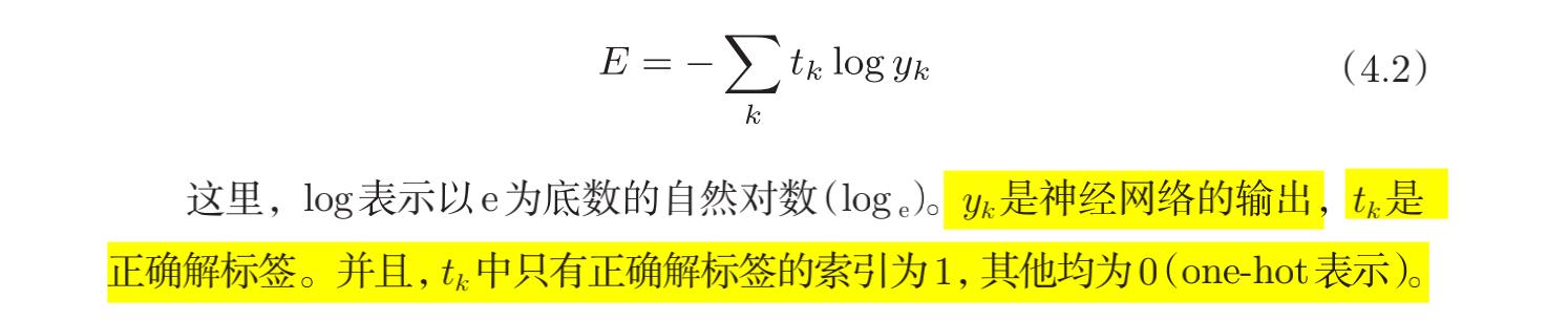
    grad = numerical_gradient(function_2, np.array([X, Y]) )
    
    plt.figure()
    plt.quiver(X, Y, -grad[0], -grad[1],  angles="xy",color="#666666")#,headwidth=10,scale=40,color="#444444")
    plt.xlim([-2, 2])
    plt.ylim([-2, 2])
    plt.xlabel('x0')
    plt.ylabel('x1')
    plt.grid()
    plt.legend()
    plt.draw()
    plt.show()

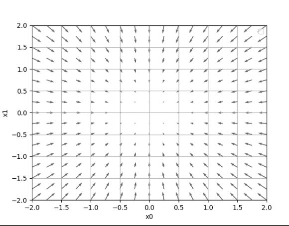
使用梯度下降求解$f(x)=x_0^2+x_1^2$的最小值

# coding: utf-8
import numpy as np
import matplotlib.pylab as plt
from gradient_2d import numerical_gradient


def gradient_descent(f, init_x, lr=0.01, step_num=100):
    x = init_x
    x_history = []

    for i in range(step_num):
        x_history.append( x.copy() )

        grad = numerical_gradient(f, x)
        x -= lr * grad

    return x, np.array(x_history)


def function_2(x):
    return x[0]**2 + x[1]**2

init_x = np.array([-3.0, 4.0])    

lr = 0.1
step_num = 20
x, x_history = gradient_descent(function_2, init_x, lr=lr, step_num=step_num)

plt.plot( [-5, 5], [0,0], '--b')
plt.plot( [0,0], [-5, 5], '--b')
plt.plot(x_history[:,0], x_history[:,1], 'o')

plt.xlim(-3.5, 3.5)
plt.ylim(-4.5, 4.5)
plt.xlabel("X0")
plt.ylabel("X1")
plt.show()

个人理解

求一个函数在某一点的斜率

比如 $f(x)=0.01x^2+0.1x$在点$x=5$的斜率

# coding: utf-8
import numpy as np
import matplotlib.pylab as plt

# 计算f(x)在x的斜率
def numerical_diff(f, x):
    h = 1e-4 # 0.0001
    return (f(x+h) - f(x-h)) / (2*h)


# 定义f(x)
def function_1(x):
    return 0.01*x**2 + 0.1*x 


# 返回f(x)在点x的切线方程
def tangent_line(f, x):
    # d:斜率
    d = numerical_diff(f, x)
    print(d)
    # y:偏移量
    y = f(x) - d*x
    return lambda t: d*t + y
     
x = np.arange(0.0, 20.0, 0.1)
y = function_1(x)
plt.xlabel("x")以上是关于《深度学习入门 基于Python的理论与实现》书中代码笔记的主要内容，如果未能解决你的问题，请参考以下文章
 
 《深度学习入门：基于Python的理论与实现》高清中文版PDF+源代码
 《深度学习入门：基于Python的理论与实现》高清中文版PDF+源代码
 分享《深度学习入门：基于Python的理论与实现》高清中文版PDF+源代码
 分享《深度学习入门：基于Python的理论与实现 》中文版PDF和源代码
 《深度学习入门基于Python的理论与实现》pdf下载在线阅读，求百度网盘云资源
 对比学习资料《深度学习入门:基于Python的理论与实现》+《深度学习原理与实践》+《深度学习理论与实战基础篇》电子资料